Table of Contents
Non-parametric probability density estimation - Parzen window
As in the previous lab, we are again interested in probability density $p_{X|k}(x|k)$ estimation. Sometimes, however, one is challenged with the problem of estimating the probability density function without even knowing its parametric form (cf MLE labs). In such cases, non-parametric estimation using Parzen window method [1] can be applied.
The kernel density estimation $\hat{f}_h(x)$ of an unknown distribution $f(x)$ given a set $\{x_1, \ldots, x_n\}$ of independent identically distributed (i.i.d) measurements is defined as $$ \hat{f}_h(x) = \frac{1}{n}\sum_{i=1}^n K_h(x - x_i) $$ where $K_h$ is the kernel (a symmetric function that integrates to one) and $h$ is the kernel size (bandwidth). Different kernel functions can be used (see [1]), but we will use $K_h(x) \equiv N(0, h^2)$, i.e. the normal distribution with mean 0 and standard deviation $h$.
Please, note that the kernel parameter $h$ does not make the method “parametric”. The parameter defines smoothness of the estimate, not the form of the estimated distribution. Nevertheless, the choice of $h$ still influences the quality of the estimate as you will see below. Using cross-validation [4] we will find such value of $h$ that ensures the estimate generalises well to previously unseen data.
Finally, using the above estimates of the probability density functions $p_{X|k}(x|k)$, we will once again build a Bayesian classifier for two letters and test it on an independent test set.
To fulfil this assignment, you need to submit these files (all packed in a single .zip file) into the upload system:
answers.txt- answers to the Assignment Questionsassignment_05.m- a script for data initialisation, calling of the implemented functions and plotting of their results (for your convenience, will not be checked)my_parzen.m- Parzen window estimatorcompute_Lh.m- function for computing cross-validated log-likelihood ratio as a function of $h$classify_bayes_parzen.m- classification using Parzen window density estimatesparzen_estimates.png- plots of estimates of $p_{X|k}(x|A)$ for varying $h$optimal_h_classA.png,optimal_h_classC.png- graph with optimal bandwidth $h$ for class A and C respectively
Start by downloading the template of the assignment. When preparing the archive file for the upload system, do not include any directories, the files have to be in the archive file root.
Information for development in Python
Experimental. Use at your own risk.
Standard is to use Matlab. You may skip this info box if you follow the standard rules.
General information for Python development.
To fulfil this assignment, you need to submit these files (all packed in a single .zip file) into the upload system:
answers.txt- answers to the Assignment Questionsparzen.ipynb- a script for data initialization, calling of the implemented functions and plotting of their results (for your convenience, will not be checked)parzen.py- containing the following implemented methods:my_parzen- Parzen window estimatorcompute_Lh- function for computing cross-validated log-likelihood ratio as a function of $h$classify_bayes_parzen- classification using Parzen window density estimates
parzen_estimates.png- plots of estimates of $p_{X|k}(x|A)$ for varying $h$optimal_h_classA.png,optimal_h_classC.png- graph with optimal bandwidth $h$ for class A and C respectively
Use template of the assignment. When preparing the archive file for the upload system, do not include any directories, the files have to be in the archive file root.
The tasks, part 1: Parzen window estimation
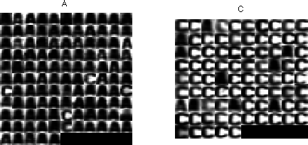
In this part we will implement the Parzen window density estimation method (see the formula above). For measurements, use the function compute_measurement_lr_cont.m from previous labs. The data loaded in the assignment_05.m template contain training data trn and test data tst - images and their correct labels. For both, the label 1 denotes an image of letter 'A' and label 2 an image of letter 'C'.
Do the following:
- For each image from the training set
trncompute the measurement $x$. Store the measurements for different classes separately, i.e. create two vectorsxAandxC.
- Complete the template of the function
p = my_parzen(x, trn_x, h)so that for a given $x$ (possibly a vector of values) it computes the Parzen estimation of probability density $p_{X|k}(x|k)$. Here,trn_xis a vector of training measurements for one of the classes (xAorxC) and $h$ is the kernel bandwidth. As the kernel function $K_h(x)$ use the normal distribution $N(0, h^2)$.
Hint: Usenormpdf()to calculate $K_h$.
p = my_parzen([1 2 3], [-1 0 2 1.5 0], 1);
p = [0.2264    0.1727    0.0761];
- Use
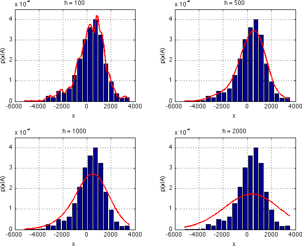
my_parzenfunction to estimate the probability distribution $p_{X|k}(x|A)$. Show the normalised histogram ofxAand the estimated $p_{X|k}(x|A)$ for $h \in \{100, 500, 1000, 2000\}$ in one figure (usesubfigurefunction) and save it asparzen_estimates.png.- To compute the estimate of $p_{X|k}(x|A)$ use your function: $p_{X|k}(x|A)$ =
my_parzen(x, xA, h) - Iterate the variable $x$ e.g. from
min(xA)tomax(xA), with a step of 100.
The tasks, part 2: Finding the optimal kernel size
As we have just seen, different values of $h$ produce different estimates of $p_{X|k}(x|A)$. Obviously, for $h=100$ the estimate is influenced too much by our limited data sample and it will not generalise well to unseen examples. For $h=2000$, the estimate is clearly oversmoothed. So, what is the best value of $h$?
To assess the ability of the estimate to generalise well to unseen examples we will use 10-fold cross-validation [4]. We will split the training set ten times (10-fold) into two sets $X^i_{\mbox{trn}}$ and $X^i_{\mbox{tst}}$, $i=1,\ldots,10$ and use the set $X^i_{\mbox{trn}}$ for distribution estimation and the set $X^i_{\mbox{tst}}$ for validation of the estimate. We will use the log-likelihood of the validation set given the bandwidth $h$, $L^i(h) = \sum_{x\in X^i_{\mbox{tst}}} log(p_{X|k}(x|A))$, averaged over ten splits $L(h)=1/10 \sum_{i=1}^{10} L^i(h)$ as a measure of the estimate quality. The value of $h$ which maximises $L(h)$ is the one which produces an estimate which generalises the best. See [4] for further description of the cross-validation technique.
Do the following:
- Estimate the optimal value of the bandwidth $h$ using the 10-fold cross-validation. The procedure (shown for the class A, the class C is analogous) is as follows:
- Split the training set
xAinto 10 subsets using thecrossvalfunction (the one from the STPR toolbox!).
- Complete the template function
Lh = compute_Lh(itrn, itst, x, h).
The function needs to compute the log-likelihood $L^i(h)$ on the each pair of training and test sets $X^i_{\mbox{trn}}$ (itrn{i}) and $X^i_{\mbox{tst}}$ (itst{i}) using the training part for estimation of $p_{X|k}(x|A)$ and the test part for computing the log-likelihood. The output is the mean log-likelihood $L(h)$ over all 10 folds.
Hint: $p_{X|k}(x|A) = \mbox{my_parzen}(x, X^i_{\mbox{trn}}, h)$.
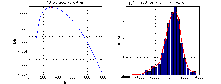
- Plot the log-likelihood average $L(h)$ for $h = 100, 150, \ldots, 1000$. Find the optimal value of $h$ using the
fminbndfunction and show the density estimate of $p_{X|k}(x|A)$ with the optimal $h$. Save the graphs intooptimal_h_classA.png
Hint: Use the functionsubfigure
- Repeat the previous steps to estimate the distribution of $p_{X|k}(x|C)$ (save the figure into
optimal_h_classC.png.
- Use the estimated distributions $p_{X|k}(x|A)$ and $p_{X|k}(x|C)$ to create a Bayesian classifier with zero-one loss function:
- Estimate the a priori probabilities $p_K(A)$ and $p_K(C)$ on the training set, as you did last week.
- Complete the template of the function
labels = classify_bayes_parzen(x_test, xA, xC, pA, pC, h_bestA, h_bestC)which takes the measurementsx_testcomputed on settstand finds a label for each test example.
Hint: Notice, thatmy_parzenreturns a probability for any $x$, also for $x\in \mbox{x_tst}$. No need for approximation, interpolation or similar techniques here!
Assignment Questions
Fill the correct answers to your answers.txt file.
For the following questions it is assumed you run rand('seed', 42); always before the splitting of the training set (for both A and C). Subsequent uses of the random generator (including crossval function) will be unambiguously defined.
- Is it possible to estimate $p_{X|k}(x|k)$ outside of the range of the [min(x_trn), max(x_trn)] interval?
- a) Yes
- b) No
- c) Only if we have enough data
- What is the optimal value of $h$ for class A and class C rounded to two decimal points?
- What is the classification error (in percents) of the Bayesian classifier rounded to two decimal points?
Bonus task
Adapt your code to accept two dimensional measurements
- x = (sum of pixel intensities in the left half of the image) - (sum of pixel intensities in the right half of the image)
- y = (sum of pixel intensities in the top half of the image) - (sum of pixel intensities in the bottom half of the image)
The kernel function will now be a 2D normal distributions with diagonal covariance matrix cov = sigma^2*eye(2). Display the estimated distributions $p_{X|k}(x|k)$.
References
- [1] Parzen window
- [3] Parzen Windows Method (V. Hlaváč) in Czech
- [4] Cross-validation