Table of Contents
Maximum Likelihood Parameter Estimation
At the very beginning of the recognition labs, we assumed the conditioned measurement probabilities $p_{X|k}(x|k)$ and the a priori probabilities $P_K(k)$ to be known and we used them to find the optimal Bayesian strategy. Later, we looked at problems where the a priori probability is not known or does not exist and we constructed the optimal minimax strategy. Today, we face the problem of unknown probability density function $p_{X|k}(x|k)$ and we will be interested in its estimation.
Lets assume in this lab that we know the density function is from a class of functions parametrised by unknown parameters. In our case, the known model is going to be Normal distribution and all we do not know are its parameters - mean and standard deviation. To estimate the parameters we will use so called training examples (training set) - a set of examples drawn randomly from some existing but unknown distribution.
The assignment has two parts. In the first one we will explore the importance of the sufficient training set size. We will see what happens if we do not have enough training examples for the estimate. In the second part, we will continue with the letter classification task and we will train a Bayes classifier using training sets of different sizes and we will focus on maximising the likelihood function.
To fulfil this assignment, you need to submit these files (all packed in a single .zip file) into the upload system:
answers.txt- answers to the Assignment Questionsassignment_04.m- a script for data initialization, calling of the implemented functions and plotting of their results (for your convenience, will not be checked)mle_normal.m- function for estimating the parameters of a normal distribution from a training setmle_variance.m- function for computing the estimate variance over 100 random training setsestimate_prior.m- functions for computing the prior probability of a given classloglikelihood_sigma.m- functions which computes the log-likelihood for a given class with arbitrary sigma valuesmle_variances.png- the graf of estimate variance as a function of the training set sizeloglikelihood20.png,loglikelihood200.png,loglikelihood2000.png- images of log likelihood for different training sizesmle_estimatesA.png,mle_estimatesC.png- images of estimated distributions for class A and Cmle_classif20.png,mle_classif200.png,mle_classif2000.png- classification results for our three estimates
Start by downloading the template of the assignment.
Information for development in Python
Experimental. Use at your own risk.
Standard is to use Matlab. You may skip this info box if you follow the standard rules.
General information for Python development.
To fulfil this assignment, you need to submit these files (all packed in a single .zip file) into the upload system:
answers.txt- answers to the Assignment Questionsmle.ipynb- a script for data initialization, calling of the implemented functions and plotting of their results (for your convenience, will not be checked)mle.py- containing the following implemented methods:mle_normal- function for estimating the parameters of a normal distribution from a training setmle_variance- function for computing the estimate variance over 100 random training setsestimate_prior- functions for computing the prior probability of a given classloglikelihood_sigma- functions which computes the log-likelihood for a given class with arbitrary sigma values
mle_variances.png- the graf of estimate variance as a function of the training set sizeloglikelihood20.png,loglikelihood200.png,loglikelihood2000.png- images of log likelihood for different training sizesmle_estimatesA.png,mle_estimatesC.png- images of estimated distributions for class A and Cmle_classif20.png,mle_classif200.png,mle_classif2000.png- classification results for our three estimates
Use template of the assignment. When preparing the archive file for the upload system, do not include any directories, the files have to be in the archive file root.
Tasks, part 1: About the training set size
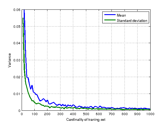
First we use a synthetic experiment to demonstrate the effect of the training set size on the parameter estimate. We will generate random training sets of different sizes from the normal distribution (using randn function) and for each set we do the maximum likelihood estimate of mean and standard deviation parameters. For each training set size we will repeat the estimate 100x and we will measure the “stability” of the estimate by variance over these 100 estimates.
Do the following:
- Complete the template function
[mu sigma] = mle_normal(x)so that for given training set it returns the maximum likelihood estimates of mean and standard deviation of a normal distribution.
Hint: The closed form solution for the maximum likelihood estimator with normal distributions is explained in [2]. Do not use MATLAB functionsmean,stdandvarin this assignment at all.
x = [0 1 2 3 4 5 6 7 8 9 10];
[mu sigma] = mle_normal(x)

mu = 5
sigma = 3.1623
- Complete the template function
[var_mean var_sigma] = mle_variance(cardinality)which for given training set size generates randomly (using therandnfunction) 100 training sets of that size, callsmle_normalon each of them and returns the variance of the estimated mean and standard deviation.
Hint 1: Generate the data from N(0,1) as done by default byrandnfunction.
Hint 2: Do not specify the random seed in any way, so that we can test the code.
Hint 3: Do not use the MATLABvarorstdfunctions, use the expression from point 1.
- Plot the estimate variances for various training set sizes into one graph and save it as
mle_variances.png.
Hint: Graphs depend on the random generator seed and may differ.
Tasks, part 2: Building a classifier
We will keep on solving the letters classification task. However, in contrast to the previous labs, both, the a priori probabilities $p_{K}(k)$ and the conditional probability density functions $p_{Xk}(x|k)$ are unknown. We have a set of training images from which the probabilities can be estimated and test examples (test set) to verify our estimate.
To estimate $p_{X|k}(x|k)$ we assume that a normal distribution fits the data, $p_{X|k}(x|k) \sim N(\mu_k, \sigma_k)$, and we compute its parameters $\mu_k$, $\sigma_k$ with the maximum likelihood criteria. Here, the $k$ is the class label - the letter we consider. The a priori probability of each class can be simply estimated by taking the fraction of the training images belonging to this class.
Having estimated the a priori probabilities and the conditional probability density functions we can use the Bayesian classifier to solve the problem.
The performance of the classifier will be measured with the classification error using a different set of pre-labelled images called test set, which was not used in the training stage. We will work with three different training sets of images (20, 200 and 2000 images) so we can experiment with the performance of the classifier, i.e. observing the classification error, when the set size changes.
As before, the following simple measurement will be used during the task:
x = (sum of pixel values in the left half of image)
   -(sum of pixel values in the right half of image)
as implemented in
x = compute_measurement_lr_discrete(imgs).
Do the following:
- Load the data file
data_33rpz_cv04.matinto Matlab. Three image sets for training are available,trn_20,trn_200andtrn_2000with 20, 200 and 2000 pre-labelled images.
- For all the training sets do the following:
- Estimate the prior probabilities $p_{K}(A)$ and $p_{K}(C)$. For this, complete the template
prior = estimate_prior(idLabel, labelling).
labelling = [1 1 1 0 0 0 0 0 0];
prior = estimate_prior(1, labelling)

prior = 0.3333
- Compute the parameters $\mu_k$ and $\sigma_k$ of the conditional distributions $p_{Xk}(x|A)$ and $p_{Xk}(x|C)$, with the maximum likelihood estimator using the
[mu sigma] = mle_normal(x)function implemented in the first part.
- Complete the template
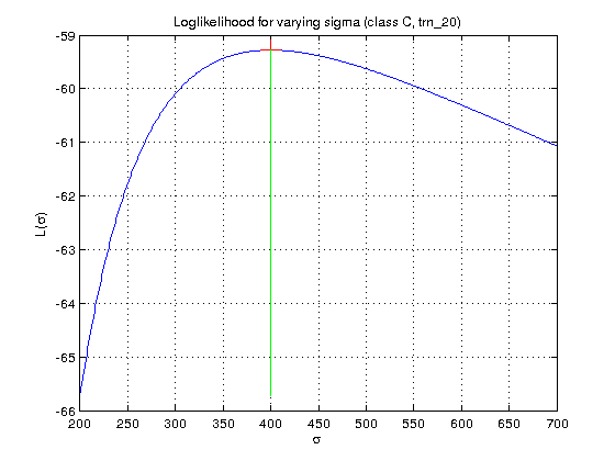
[L maximizerSigma maxL] = loglikelihood_sigma(x, D, sigmas)which for fixed $\mu_k$ computed in 2.II computes the log-likelihood functionLas a function of $\sigma_k$. The function should also return the $\sigma^*_k$ corresponding to the maximum of the log-likelihood function.
Hint: $L$ is defined in equation (2) in [2] (or [1], eq 5, page 87).
Hint: Use the same function as in the last assignment to find a maximum of a function:x_maximizer = fminbnd(@(x) -some_function(other_param1, other_param2, x), 0, 1)
Hint: Derive the log-likelihood expression (using pen and paper) and use this in your code to avoid precision errors coming from first exponentiating and then taking logarithm (Example of such problem:exp(-x^2/2)evaluates to0for values ofxas low asx=40. Takinglogof that produces-Inf. But using-x^2/2(manually derived log of exp) instead avoids that. Using log of MATLAB normpdf can cause similar problems.sigmas = 300:50:3500; x = compute_measurement_lr_cont(trn_2000.images); D.Mean = -2000; [L maximizerSigma maxL] = loglikelihood_sigma(x, D, sigmas); maximizerSigma = 2.1247e+03 maxL = -1.6345e+04
- Plot the computed log-likelihood as a function of $\sigma_k$ for $k=A$ and save it into
loglikelihoodXXX.png(XXX corresponds to the training set size, i.e. 20, 200, or 2000)
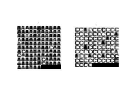
- Plot all the estimates of $p_{Xk}(x|A)$ and $p_{Xk}(x|C)$ from different training set sizes into one graph together with normalised histogram of the
trn_2000images. Save this asmle_estimatesA.pngandmle_estimatesC.png.


- Use the estimates to build a Bayesian classifier (use your implementation from the previous labs) assuming zero-one loss function. Apply the classifier to the test set and compute the classification error (notice, that the question 2 below asks for this number).
- Show the final classification in one figure and save it as
mle_classifXXX.png(again, XXX is either 20, 200 or 2000).


Assignment Questions
Fill the correct answers to your answers.txt file.
- Is it true that with a higher number of samples in the training set we get more accurate parameter estimates?
- a) Yes
- b) No
- c) Not necessarily but it is more likely
- What is the classification error for the test set given the maximum likelihood estimates from
trn_20,trn_200andtrn_2000(rounded to three decimal points)? Use the following syntax:
question2 : [1.001, 2.002, 3.003]
Bonus Task
Implement ML estimation of a bivariate normal distribution.
- Load the data file
data_33rpz_cv04.mat. - Compute 2 dimensional features <latex>X = (x, y)^T</latex> as in the Bayes assignment. Use the
trn_2000training set. - Estimate parameters of bivariate normal distributions $$f_k(\mathbf x) = \frac{1}{\sqrt{(2\pi)^2|\boldsymbol\Sigma_k|}} \exp\left(-\frac{1}{2}({\mathbf x}-{\boldsymbol\mu_k})^T{\boldsymbol\Sigma_k}^{-1}({\mathbf x}-{\boldsymbol\mu_k}) \right)$$ for classes $ k \in \{A,C\} $:
- $\boldsymbol\mu_k$ mean vectors
- $\boldsymbol\Sigma_k$ covariance matrices - do not use
covfunction to calculate covariance matrix, you can take advantage of matrix multiplication, see Estimation_of_covariance_matrices#Estimation_in_a_general_context.
- Build Bayes classifier (use already computed priors $p_{K}(A)$ and $p_{K}(C)$), classify
tsttest data and display the results as in the main assignment above. - Display the distribution estimates (use the function
pgauss) and the test set (functionppatterns).


Recommended Literature
- [1] Richard O. Duda, Peter E. Hart, David G. Stork. Pattern Classification.
- [2] Maximum Likelihood Parameter Estimation (short support text for labs)
- [3] Maximálně věrohodný odhad (longer text in Czech, includes multi-dimensional normal distribution estimates (13,14) needed for bonus task)