Table of Contents
Image intensity transforms
In this lab, the following topics will be dealt with:
- histogram
- cumulative distribution function (CDF)
- quantiles of a distribution
- histogram equalization
- constrained histogram equalization
- histogram matching
All of these will be employed to find useful image intensity transformations which will either normalize an image, or will make it better suited for viewing.
Note the following conventions used in this assignment:
- Images are stored by float (single or double) matrices, and are normalized to $[0, 1]$ range.
- Discretized 1D functions of an intensity range $[0, 1]$ are stored in row vectors by function values ('$y$-values') only. This includes histogram(s), CDF(s), or look-up-tables (LUTs). It is understood that the corresponding domain intensity values ($x$-values) can be obtained from a row vector by the following considerations:
- first element in the vector corresponds to intensity $x=0$
- last element in the vector corresponds to $x=1$
- the stepping between these two limits is uniform.
- Thus, for a vector
h, the corresponding intensity valuesxcan be obtained by
x = linspace(0, 1, length(h));
Histograms and CDFs

% create an array of the capital letters
letters = 'ABCDEFGHIJKLMNOPQRSTUVWXYZ';

% create a 20 by 20 matrix of random integers from 1 to 26 (i.e. the length of the alphabet)
numMat = randi(length(letters), 20, 20);

subplot(2, 3, 1);
% this can be thought of as a gray-scale image, let's plot it as such
imshow(numMat ./ length(letters), [0 1]);
colormap(gca, 'gray')
title('Gray-scale image from the numeric matrix')

% compute histogram of the values contained in the matrix
numHist = hist(numMat(:), 26);

subplot(2, 3, 2);
colormap('default')
% numHist variable holds the individual counts or occurrences of the values in the matrix
bar(numHist);
title('Histogram of the numeric matrix');
xlim([1 length(letters)]);
ax = gca;
ax.XTick = 1:length(letters);

% let's create a matrix of letters from the numeric matrix, by substituting the integers with letters
letterMat = letters(numMat);

% manually count the occurrences of the individual letters
letterHist = zeros(1, length(letters));
for l = letters
    lpos = find(letters == l);
    letterHist(lpos) = sum(sum(l == letterMat));
end

subplot(2, 3, 3);
% variable letterHist holds the counts of the individual letters in the alphabetic matrix
bar(letterHist);
title('Histogram of the alphabetic matrix');
xlim([1 length(letters)]);
ax = gca;
ax.XTick = 1:length(letters);
ax.XTickLabel = letters';

% CDFs
subplot(2, 3, 5);
% CDF can be computed from a histogram by calculating the cumulative sum of the histogram
plot(cumsum(numHist));
title('CDF of the numeric matrix');
xlim([1 length(letters)]);
ax = gca;
ax.XTick = 1:length(letters);

subplot(2, 3, 6);
% the same procedure as before, just with the alphabetic histogram
plot(cumsum(letterHist));
title('CDF of the alphabetic matrix');
xlim([1 length(letters)]);
ax = gca;
ax.XTick = 1:length(letters);
ax.XTickLabel = letters';
Start by downloading the template of the assignment. It contains function templates and the data needed for the tasks.
Getting started
Change to the directory where you unzipped the archive. Have a close look onto the provided functions/templates and try to run it in Matlab. Make sure that you understand it really well. The following code is also contained in the package as the script hw_histogram_1.m.
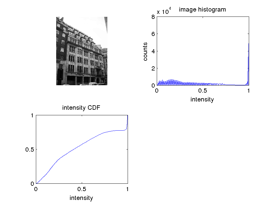
% get an image:
im = get_image('images/L.jpg');

% display it:
figure();
imshow(im);

% get histogram and CDF:
Nbins = 256;
[bin_centers, h, cdf] = image_hist_cdf(im, Nbins);

% plot histogram:
figure();
plot(bin_centers, h);
title('image histogram');

% show CDF:
figure();
plot(bin_centers, cdf);
title('intensity CDF');

% Showing these three (im, its histogram and CDF) will be quite handy
% for other tasks as well, so why not to put it to a separate
% function. Make the function yourself. It should produce the result
% similar to this one:
showim_hist_cdf(im);

% Now make a simple LUT which performs negative transform:
lut_neg = linspace(1, 0, Nbins);

% and display it:
figure();
plot(bin_centers, lut_neg);

% use it to transform im to negative:
im_neg = transform_by_lut(im, lut_neg);

% and show it:
showim_hist_cdf(im_neg);

% Note the differences with the original image its histogram and CDF.
Image enhancement by stretching the itensity range
A simple method for enhancing an image is the following: Find quantiles $x_{low}$ and $x_{high}$ for $p_{low}=0.01$ and $p_{high}=0.99$, respectively, and then map intensities $x \le x_{low}$ to 0, $x \gt x_{high}$ to 1, and values between $x_{low}$ and $x_{high}$ linearly from 0 to 1. If you imagine the pixels sorted by intensities in ascending order then this effectively means the first 1% of pixels are mapped to 0, the last 1% of pixels to 1. Note that $p_{low}$ and $p_{high}$ are the parameters of the method.
Your task is to implement the function which finds the quantiles from cdf (range_by_quantiles) and
constructs the LUT from the found range (lut_from_range).
This is how it will work. The following code is included in the package as hw_histogram_2.m.
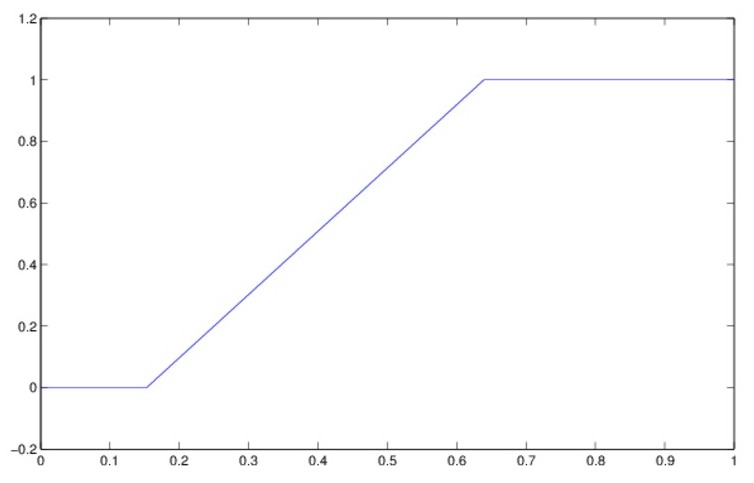
im = get_image('images/P.jpg');
Nbins = 256;
[bin_centers, h, cdf] = image_hist_cdf(im, Nbins);
showim_hist_cdf(im);

% get 1% and 99% quantile of CDF:
p_low = 0.01;
p_high = 0.99;
[x_low, x_high] = range_by_quantiles(cdf, p_low, p_high);
% Expected result:
% x_low = 0.1490
% x_high = 0.6431

% construct LUT:
lut = lut_from_range(x_low, x_high, Nbins);

% and display it:
figure();
plot(bin_centers, lut);
ylim([-0.2, 1.2]);

% apply it and show result:
im_stretched = transform_by_lut(im, lut);
showim_hist_cdf(im_stretched);
LUT:
Effect of LUT:
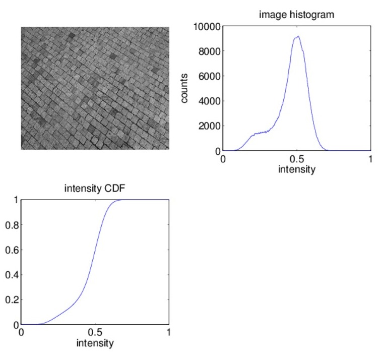 | → | 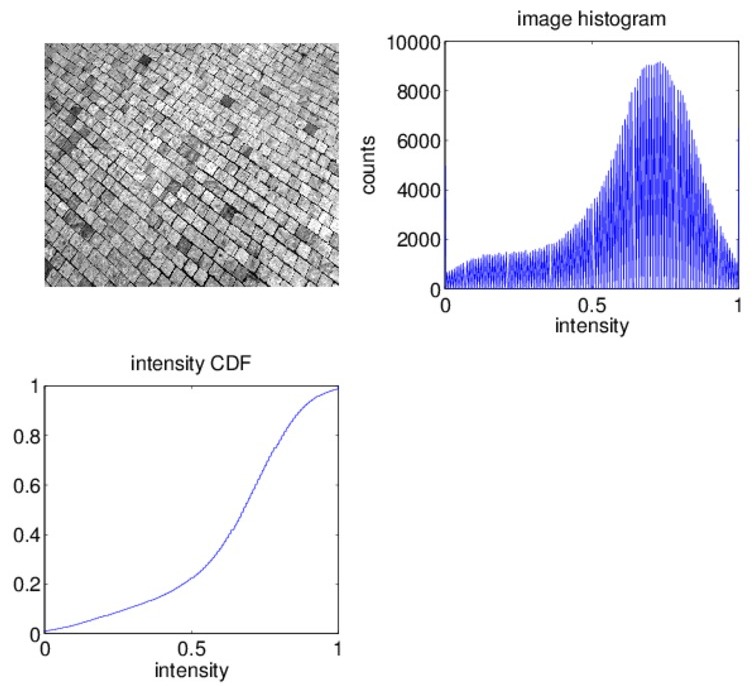 |
Implementation note: Use Matlab function interp1 while implementing lut_from_range.m. Be careful to fulfil this function requirements (e.g. non-repeating x-values). You may find Matlab function unique useful.
Unconstrained and constrained histogram equalization
im = get_image('images/L.jpg');
Nbins = 256;

% show the original image:
showim_hist_cdf(im);

% apply histogram equalization:
[bin_centers, h, cdf] = image_hist_cdf(im, Nbins);
lut_eq = hist_equalization(cdf);
im_eq = transform_by_lut(im, lut_eq);

% show the equalized image:
showim_hist_cdf(im_eq);
The unconstrained histogram equalization normalizes the image nicely, but produces artifacts (see the sky region)

The problem is that the transformation produced by histogram equalization is too steep at some points. We will implement the function constrained_lut.m which takes a LUT and changes it such that it its slope (=derivative, finite difference) is nowhere greater
than a predefined parameter max_slope. The slopes can be estimated from differences of subsequent domain values and target values of LUT:
dx = x(2) - x(1) = x(3) - x(2) = ...
slope(1) = (LUT(1) - 0) / dx = LUT(1) / dx
slope(i) = (LUT(i) - LUT(i-1)) / dx, i = 2...length(LUT)
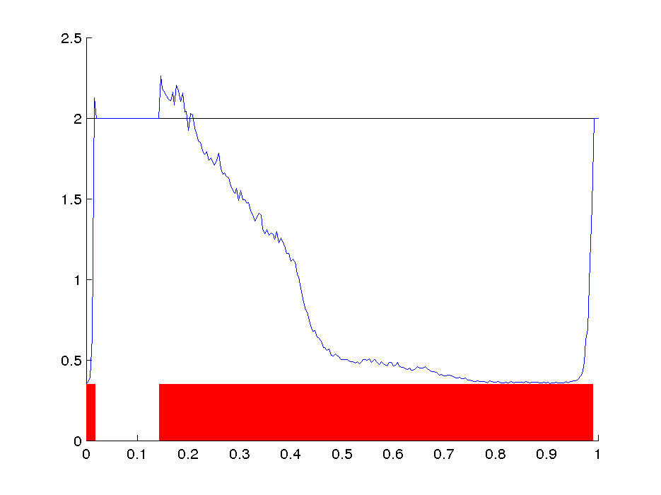
The slope limitation will be done as follows. Let us have a look at the slopes of our LUT (which is CDF in the case of histogram equalization), and consider max_slope = 2:
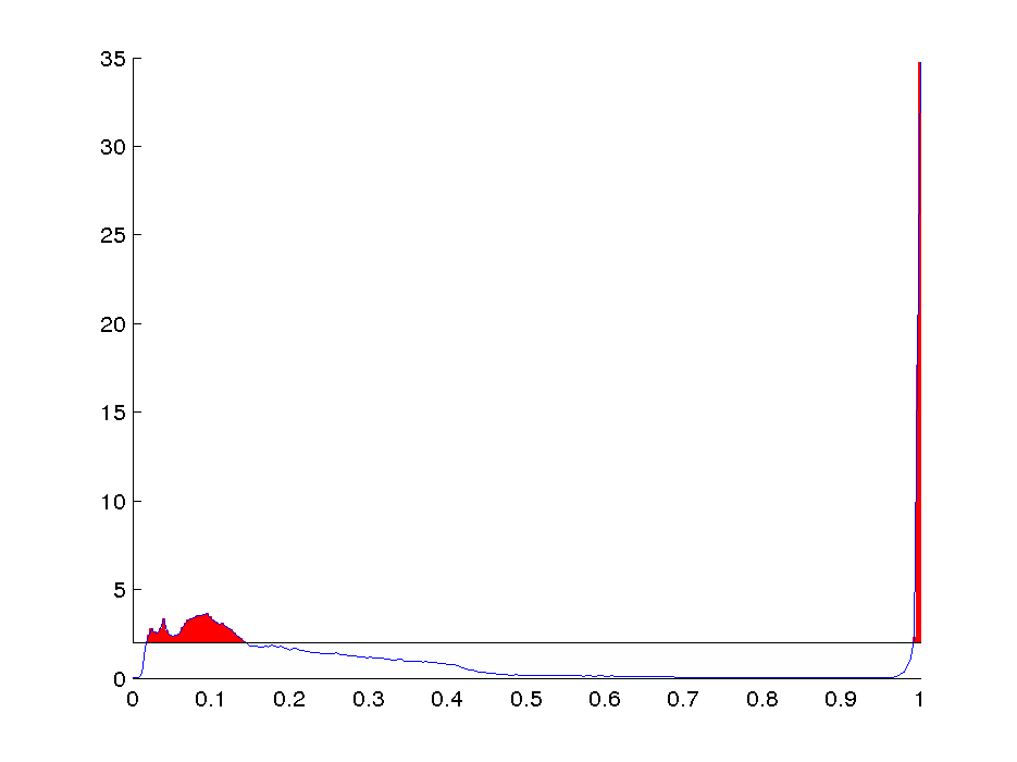
As we can see, the slopes go to values much larger than the threshold (violating parts are shown in red). We will now modify the slopes by redistributing the mass shown in red ($\ge$max_slope) uniformly to the bins which do not violate the constraint:
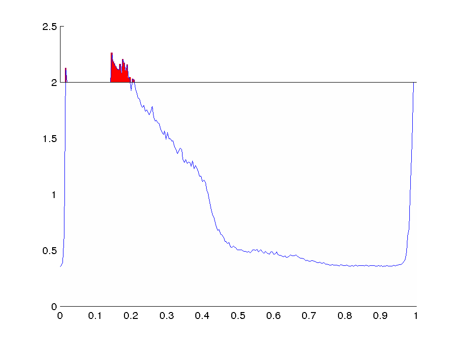
The redistribution is done so that when the slopes are integrated back to a new LUT, the right-most value does not change from the original LUT. Note that the vertical scale decreased its magnitude significantly and now almost all points fulfil the condition on slope. But by redistributing the mass, some of the bins which did not violate the constraint now do (see the left picture), and the next redistribution brings us much closer to the desired result (see right):
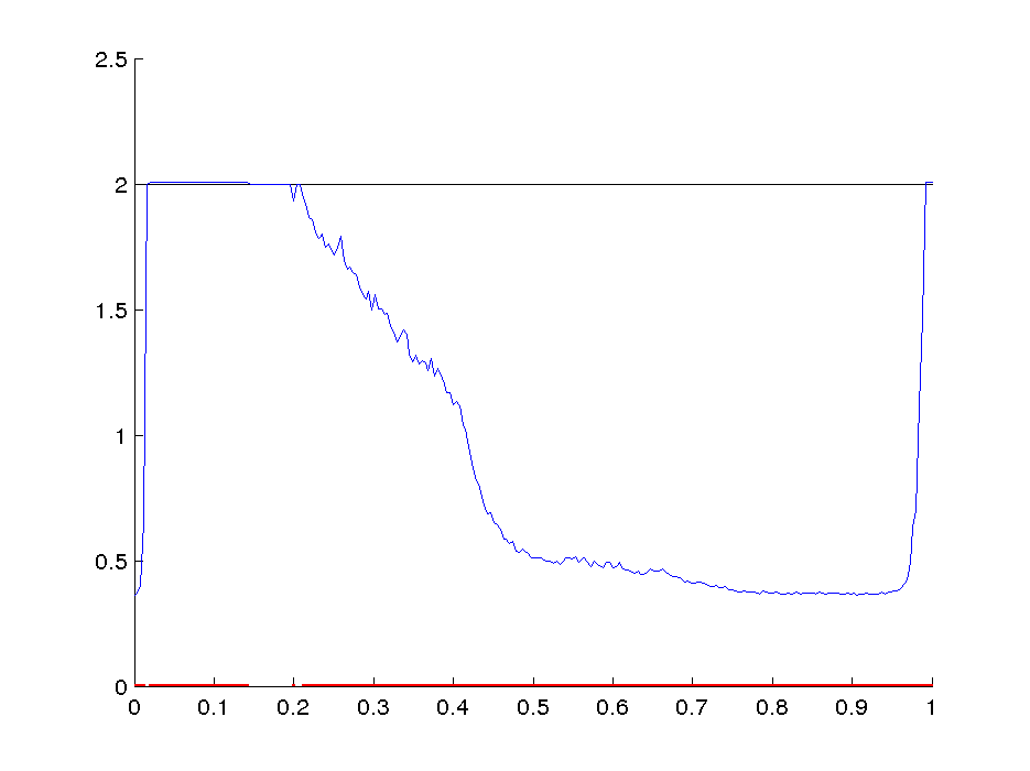
We can keep doing this until no slopes violate the constraint. This usually happens is 15-20 iterations.
Note. In this function, slopes need to be computed first from the LUT. Then, slopes are iteratively modified in order to satisfy the constraint. Finally, the slopes are again integrated into a new LUT. Note that it will be quite handy to first skip the middle part and check whether the code 1) correctly computes slopes, 2) correctly integrates them to a LUT identical to the original LUT.
Once having implemented the function constrained_lut.m, we can see it in action (continuing from equalization above). The following code is part of the script hw_histogram_3.m which is included in the package.
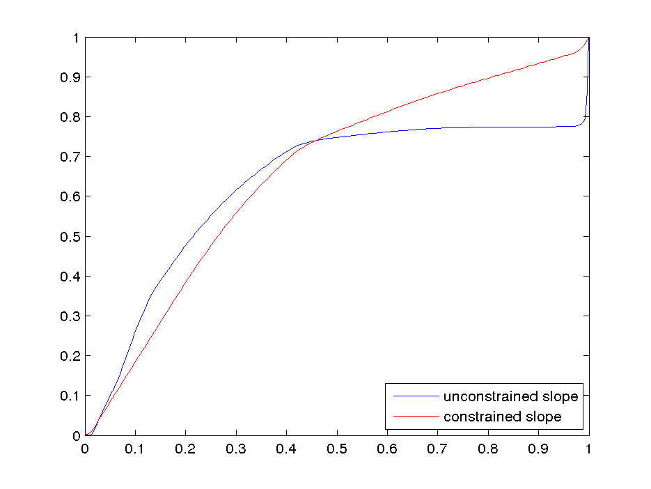
% alter the LUT by requiring limit on the slope:
max_slope = 2;
lut_eq_con = constrained_lut(lut_eq, max_slope);

% show it together with the unconstrained one:
figure();
plot(bin_centers, [lut_eq; lut_eq_con]);
ylim([0, 1]);
hlegend = legend('unconstrained slope', 'constrained slope');
set(hlegend, 'Loc', 'southeast');

% apply it:
im_eq_con = transform_by_lut(im, lut_eq_con);
showim_hist_cdf(im_eq_con);
The LUT from histogram equalization, and LUT derived from it with constraint max_slope = 2 (left). The constrained LUT applied to image (right).
Histogram matching
Have a look at these two images:
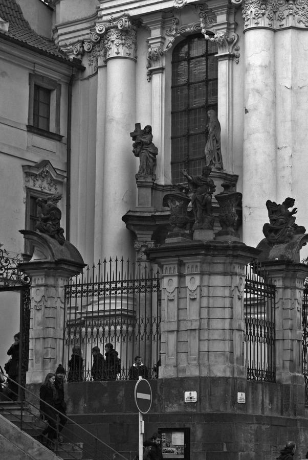

The left one was taken in October 2014, and its levels have been adjusted by hand in photo editing program. The right one was taken in October 2015 by a cheap camera and not edited in any way. We would like to bring the histogram of the second one as close as possible to the first one automatically.
Methods which do this are called histogram matching. There are several of them and we will use the one which is best suited to what we have already done.
We know that any image can be intensity-normalized by equalization. The LUT performing the equalization is approximated by CDF:
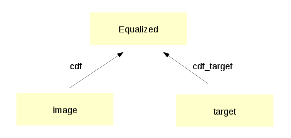
This suggests that a transformation which would make the histograms of image and target close would be the one which first transforms the image to an equalized one by LUT=cdf, and then transforms by the inverse of cdf_target. Note that composition of two LUTs can again represented by a LUT.
The core of this task is to write the function which computes the inverse of a LUT, inverse_lut.m
This is an example of its action:

Once this function is available, it is quite simple to finish the match_hists.m function.
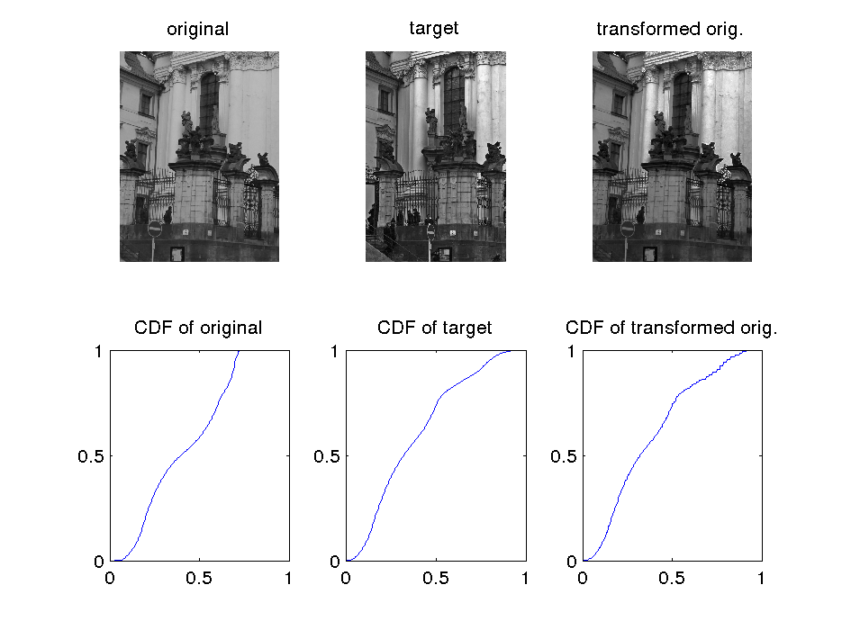
Here is an example which is also included in the package as hw_histogram_4.m.
im = get_image('images/CM1.jpg');
im_target = get_image('images/CM2.jpg');
Nbins = 256;

% get histograms of both images:
[bin_centers, h, cdf] = image_hist_cdf(im, Nbins);
[~, h_target, cdf_target] = image_hist_cdf(im_target, Nbins);

% match the histograms to find LUT:
lut = match_hists(h, h_target);

% apply LUT on the original image:
im_tr = transform_by_lut(im, lut);

[~, h_tr, cdf_tr] = image_hist_cdf(im_tr, Nbins);

figure();
subplot(2,3,1);
imshow(im);
title('original');
subplot(2,3,4);
plot(bin_centers, cdf);
title('CDF of original');
subplot(2,3,2);
imshow(im_target);
title('target');
subplot(2,3,5);
plot(bin_centers, cdf_target);
title('CDF of target');
subplot(2,3,3);
imshow(im_tr);
title('transformed orig.');
subplot(2,3,6);
plot(bin_centers, cdf_tr);
title('CDF of transformed orig.');
.zip file) into the upload system:range_by_quantiles.m: finds intensitiesx_lowandx_highgiven the CDF and p-quantile valuesp_lowandp_high, respectively.cdf, p_low, p_high → x_low, x_high
lut_from_range.m: computes a simple 3-segment LUT used for stretching the intensity range. LUT has N elements.x_low, x_high, N → lut
constrained_lut.m: creates an output LUT which has a limited slope (derivative), and is close to the given input lut.- lut_in, max_slope → lut_out
inverse_lut.m: for an input LUT, computes the inverse of it.- lut_in → lut_out
match_hists.m: creates a LUT which brings histogram of one image close to the histogram of another image.- h, h_target → lut
You will be given the following functions to get you started (you do not need to submit these):
get_image.m: reads an imagefnameto 2D matrixim. The output imageimadheres to the conventions above (range, type).- fname → im
image_hist_cdf: computes histogram and CDF of an image.- im, Nbins → bin_centers, h, cdf
showim_hist_cdf: just shows the use ofsubplotto show im, its histogram and CDF in a single Figure.- im → [None]
transform_by_lut.m: transforms a matrix with elements in range $[0, 1]$ by a LUT.- M_in, lut → M_out
hist_equalization.m: creates LUT from the image's CDF which equalizes the histogram.- cdf → lut
Implementation notes: When implementing inverse_lut.m, you will make use of the interp1 function. You must be careful to fulfil this function requirements (e.g. non-repeating x-values, query for interpolated values inside the range given by the minimum and maximum x-value). Once you have this function, you can finish the template for match_hists.m by adding two lines of code: one will compute the inverse of the target CDF, and the other one will combine the CDF of original image and the inverse of the target CDF to a single LUT (note that transform_by_lut can be used for this.)
Assignment deadline
Monday 23.10.2017, 23:59
Please note: Do not put your functions into any subdirectories. That is, when your submission ZIP archive is decompressed, the files should extract to the same directory where the ZIP archive is. Upload only the files containing functions implemented by yourself, both the required and supplementary ones.