Table of Contents
Logistic regression
In this labs we will build a logistic regression model for a letter (digit) classification task. It has been shown at the lecture that for many practical problems, the log odds $a(x)$ can be written as a linear function of the input $x$ $$ a(x) = \ln\frac{p_{K|x}(1|x)}{p_{K|x}(2|x)} = w\cdot x\;, $$ where the original data vector $x$ has been augmented by adding 1 as its first component (corresponding to the bias in the linear function). It follows that the aposteriori probabilities have then the form of a sigmoid function acting on a linear function of $x$ $$ p_{K|x}(k|x) = \frac{1}{1+e^{-kw\cdot x}} = \sigma(kw\cdot x)\qquad k\in\{-1, +1\}. $$ The task of estimating the aposteriori probabilities then becomes a task of estimating their parameter $w$. This could be done using the maximum likelihood principle. Given a training set $\mathcal{T} = \{(x_1, k_1), \ldots, (x_N, k_N)\}$, ML estimation leads to the following problem: $$ w^* = \arg\min_w E(w), \qquad \mbox{where}\\ E(w) = \frac{1}{N}\sum_{(x,k) \in \mathcal{T}}\ln(1+e^{-kw\cdot x})\;, $$ The normalisation by the number of training samples helps to make the energy, and thus the gradient step size, independent of the training set size.
We also know that there is no close-form solution to this problem, so a numerical optimisation method has to be applied. Fortunately, the energy is a convex function, so any convex optimisation algorithm could be used. We will use the gradient descent method in this labs for its simplicity, however, note that many faster converging methods are available (e.g. the heavy-ball method or the second order methods).
Information for development in Python
General information for Python development.
To fulfil this assignment, you need to submit these files (all packed in a single .zip file) into the upload system:
logreg.ipynb- a script for data initialization, calling of the implemented functions and plotting of their results (for your convenience, will not be checked)logreg.py- containing the following implemented methods:logistic_loss- a function which computes the logistic losslogistic_loss_gradient- a function for computing the logistic loss gradientlogistic_loss_gradient_descent- gradient descent on logistic lossget_threshold- analytical decision boundary solution for the 1D caseclassify_images- given the log. reg. parameters, classifies the input data into {-1, +1}.
E_progress_AC.png,w_progress_2d_AC.png,aposteriori.png,classif_AC.png,E_progress_MNIST,classif_MNIST.png- images specified in the tasks
Use template of the assignment. When preparing a zip file for the upload system, do not include any directories, the files have to be in the zip file root.
Task 1: Letter classification
The first task is to classify images of letters 'A' and 'C' using the following measurement:
x = normalise( (sum of pixel values in the left half of image)
              -(sum of pixel values in the right half of image))
as implemented in compute_measurements(imgs, norm_parameters). For numerical stability, the function normalises the measurements to have a zero mean and unit variance. In this first task, the measurement is one dimensional which allows easy visualisation of the progress and the results.
Tasks
- Load the data from
data_logreg.npz. It containstrnandtstdictionaries containing training and test data and their labels respectively. Augment the data so that their first component is 1. - Complete the function
loss = logistic_loss(X, y, w)which computes the energy $E(w)$ given the data $X$, their labels $y$ and some solution vector $w$.loss = logistic_loss(np.array([[1, 1, 1],[1, 2, 3]]), np.array([1, -1, -1]), np.array([1.5, -0.5])) print(loss) # -> 0.6601619507527583
- Implement the function
g = logistic_loss_gradient(X, y, w)which returns the energy gradient $g$ given some vector $w$.
Hint: Do not forget to normalise the gradient by 1/N.\\gradient = logistic_loss_gradient(np.array([[1, 1, 1],[1, 2, 3]]), np.array([1, -1, -1]), np.array([1.5, -0.5])) print(gradient) # -> [0.28450597 0.82532575]
- Next, implement the function
w, wt, Et = logistic_loss_gradient_descent(X, y, w_init, epsilon)which does the gradient descent search for the optimal solution as described in the lecture slide 21 slides. As the terminal condition use $||w_\mbox{new} - w_\mbox{prev}|| \le \mbox{epsilon}$.
Hint 1: Do not forget to add the bias component to the data.
Hint 2: Try to initialise it from different initial values of $w$ to test if it behaves as you would expect.
Hint 3: Save the candidate into $wt$ immediatelly after finding it. The distance between the last two elements of $wt$ will thus be $||wt_\mbox{last} - wt_\mbox{prelast}|| \le \mbox{epsilon}$!w_init = np.array([1.75, 3.4]) epsilon = 1e-2 [w, wt, Et] = logistic_loss_gradient_descent(train_X, trn['labels'], w_init, epsilon) print('w: ', w, '\nwt: ', wt, '\nEt: ', Et) # -> w: [1.8343074 3.3190428] # -> wt: [[1.75 1.75997171 1.77782062 1.80593719 1.83779008 1.84398609 1.8343074 ] # -> [3.4 3.39233974 3.37848624 3.35614129 3.32899079 3.31724604 3.3190428 ]] # -> Et: [0.25867973 0.25852963 0.25830052 0.25804515 0.25791911 0.25791612 0.25791452]
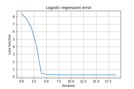
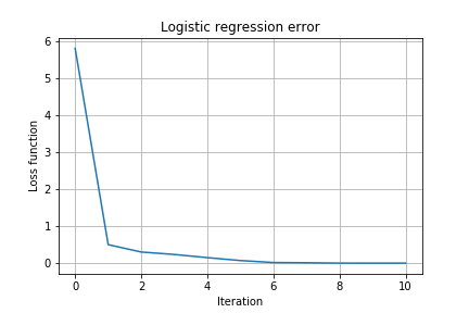
- Visualise the progress of the gradient descent:
- Plot the energy $E(w)$ in each step of the gradient descent. Save the figure into
E_progress_AC.png.
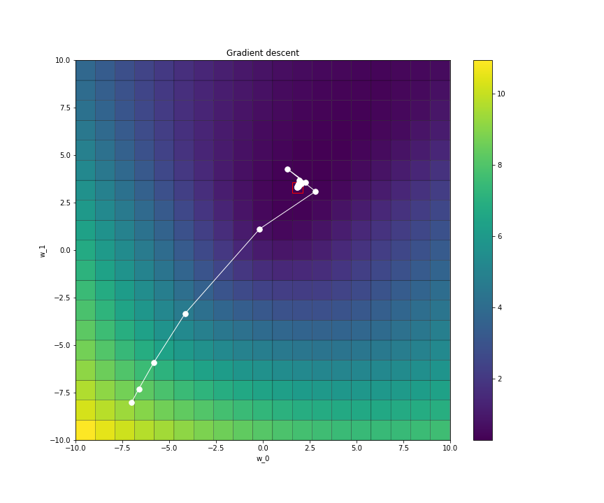
- Plot the progress of the value of $w$ in 2D (slope + bias parts of $w$) during the optimisation. For the progress of $w$ in 2D you may use the provided function
plot_gradient_descent(X, y, loss_function, w, wt, Et). Save the images asw_progress_2d_ac.png.
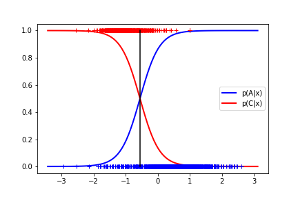
- Derive the analytical solution for the classification threshold on the (1D) data, i.e. find the x for which the aposteriori probabilities are both 0.5. Using the formula, complete the function
thr = get_threshold(w). Plot the threshold, aposteriori probabilities $p(A|x)$ and $p(C|x)$ and the training data into one plot and save the image asaposteriori.png.thr = get_threshold(np.array([1.5, -0.7])) print(thr) # -> 2.142857142857143
- Complete the function
y = classify_images(X, w)which uses the learned $w$ to classify the data in $X$.y = classify_images(np.array([[1, 1, 1, 1, 1, 1, 1],[0.5, 1, 1.5, 2, 2.5, 3, 3.5]]), np.array([1.5, -0.5])) print(y) # -> [ 1 1 1 1 1 -1 -1]
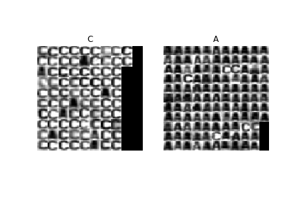
- Use the function
classify_imagesto classify the letters in thetstset. Compute the classification error and visualise the classification. Save the visualised classification results asclassif_ac.png.
Hint: Use the data normalisation returned for the training data.
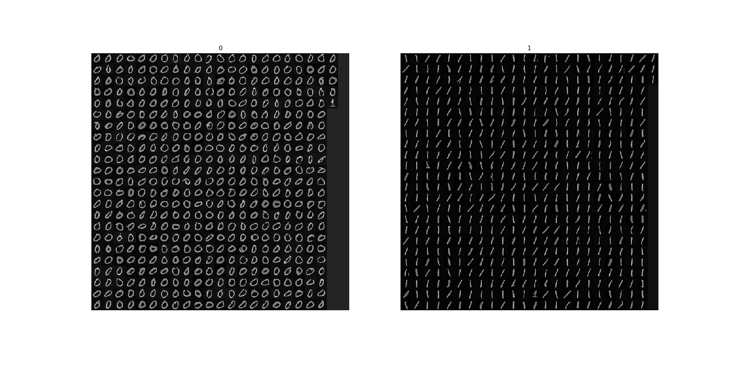
Task 2: MNIST digit classification
Next we apply the method to a similar task of digit classification. However, instead of using a one-dimensional measurement we will work directly in the 784-dimensional space (28 $\times$ 28, the size of the images) using the pixel values as individual dimensions.
Tasks
- Load the data from
mnist_trn.npz. Beware that the structure of the data is slightly different from the previous task.
- Repeat the steps from the Task 1 and produce similar outputs:
E_progress_MNIST.png,classif_MNIST.png.
Bonus task
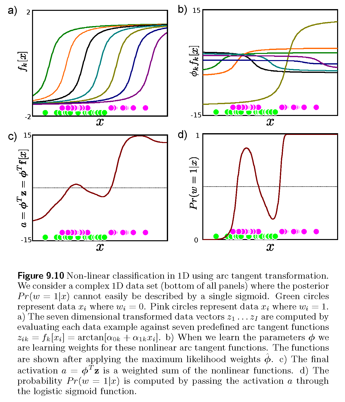
Implement the logistic regression with dimension lifting as shown in the following figure from [1]. The figure assumes $w$ being the class label and $\phi$ the sought vector. Generate similar outputs to verify a successful implementation.
References
[1] Simon J. D. Prince, Computer Vision: Models, Learning and Inference, 2012