Table of Contents
Introductory Labs
Taught competencies and skills
By attending the lab and solving the assignment, a student should…
- understand the rules of the semester.
- solve possible access problems (BRUTE, forum, KOS, …).
- be able to work with the templates.
- have experience with uploading a simple problem solution to the upload system.
To fulfill this assignment, you need to submit these files (all packed in one .zip file) into the upload system:
basics.ipynb- a script for data initialisation, calling of the implemented functions and plotting of their results (for your convenience, will not be checked).basics.py- file with implemented methods:matrix_manip- a method implementing the matrix manipulation tasks specified in the section Matrix manipulation
initial1_mean.png,initial2_mean.pngandinitials_histograms.png- images specified in the section Simple data task
Use template of the assignment. When preparing a zip file for the upload system, do not include any directories, the files have to be in the zip file root.
Beware of using for loops! :)
PYTHON introduction
We will be using the Python programming language with the NumPy library during the whole semester. Make sure you are comfortable with these so that you don't spend more time dealing with python/numpy issues than solving the assignment tasks.
For the case you are not too sure about your Python/NumPy skills, have a look here: http://cs231n.github.io/python-numpy-tutorial/, search for other materials (duckduckgo, google) or ask your teacher.
Start by reading General information for Python development and cloning the assignment template repository.
We strongly recommend using the .ipynb notebooks provided in the template. ($ pip install jupyter, then $ jupyter notebook in the directory containing basics.ipynb. Or you can use your favorite IDE jupyter notebook plugin.)
unit tests
We provide unit tests in the assignment template, see test_basics.py. To execute the tests, run $ python -m unittest.
The tests are provided to simplify local development and debugging of your code. Passing all the unit tests does not automatically mean that your code will pass all BRUTE tests, feel free to write additional tests into test_basics.py if needed. Make sure that all the unittests pass OK, before uploading to BRUTE.
Matrix manipulation with NumPy
In the first part of today’s assignment, you will start with some simple matrix manipulation tasks.
TRY TO AVOID USING LOOPS FOR MATRIX MANIPULATION IN YOUR PROGRAM! (some hints on how to do that here).
Although numpy has a matrix class, we will not be using that. Instead, we will use the array class for representing matrices, vectors, images, lists, etc. We will import numpy using
import numpy as np
Your goal is to complete a function output = matrix_manip(A, B), where A and B are input matrices (represented by np.array). The matrix_manip function should return a python dict containing the results of the operations described below.
To have some data to work with, lets use the following matrices A and B:
A = np.array([[16,  2,  3, 13],
              [ 5, 11, 10,  8],
              [ 9,  7,  6, 12],
              [ 4, 14, 15,  1]])

B = np.array([[3, 4,  9, 4, 3, 6, 6, 2, 3, 4],
              [9, 2, 10, 1, 4, 3, 7, 1, 3, 5]])
Your function should work on general input matrices, not only for the A and B shown here or for matrices with the same dimensions.
- Find the transpose of the matrix
Aand return it inoutput['A_transpose']. Example result:>> output['A_transpose'] array([[16, 5, 9, 4], [ 2, 11, 7, 14], [ 3, 10, 6, 15], [13, 8, 12, 1]])
- Select the third column of the matrix
Aand return it inoutput['A_3rd_col'].>> output['A_3rd_col'] array([[ 3], [10], [ 6], [15]])
Hint: Don't forget python and numpy use 0-based indexing. Make sure your output dimensions are correct! - Select last two rows from last three columns of the matrix A and return the matrix in
output['A_slice'].>> output['A_slice'] array([[ 7, 6, 12], [14, 15, 1]])
- Find all positions in
Agreater then 3 and increment them by 1. Afterwards add a new column of ones to the matrix (from right). Save the result tooutput['A_gr_inc'].>> output['A_gr_inc'] array([[17, 2, 3, 14, 1], [ 6, 12, 11, 9, 1], [10, 8, 7, 13, 1], [ 5, 15, 16, 1, 1]])
Hint: Try>operator on the whole matrix. The output dtype should be the same as the input dtype. Some numpy functions do not make copies of the inputs, but return 'views' of the input arrays instead. Make sure you don't corrupt the other results when computingoutput['A_gr_inc'] - Create matrix
Csuch that $C_{i,j} = \sum_{k=1}^n A\_gr\_inc_{i,k} \cdot (A\_gr\_inc^T)_{k,j}$ and store it inoutput['C'].>> output['C'] array([[499, 286, 390, 178], [286, 383, 351, 396], [390, 351, 383, 296], [178, 396, 296, 508]])
Hint: No loops are needed, use appropriate numpy matrix function. Try it on a paper with a 2×2 matrix. - Compute $\sum_{c=1}^n c \cdot \sum_{r=1}^m A\_gr\_inc_{r,c}$, store in
output['A_weighted_col_sum']:>> output['A_weighted_col_sum'] 391
Hint: Look atnp.arangeandnp.sum. Finally convert the output to Python float (as indicated in the docstring) by callingfloat(…). - Subtract a vector $(4,6)^T$ from all columns of matrix
B. Save the result to matrixoutput['D'].>> output['D'] array([[-1, 0, 5, 0, -1, 2, 2, -2, -1, 0], [ 3, -4, 4, -5, -2, -3, 1, -5, -3, -1]])
Hint: numpy broadcasting. - Select all column vectors in the matrix
D, which have greater euclidean length than the average length of column vectors inD. Store the results inoutput['D_select']>> output['D_select'] array([[ 0, 5, 0, -2], [-4, 4, -5, -5]])
Simple data task in Python
In this part of the assignment, you are supposed to work with a simple input data which contains images of letters. We will use similar data structures later on during the labs. Do the following:
- The following variables are stored in the
data_33rpz_basics.npzdata file:images(3D array of 2000 10×10 grayscale images)alphabet(letters contained in theimages, not full alphabet is included)labels(indexes of theimagesintoAlphabetarray).
- Load and access them as follows
loaded_data = np.load("data_33rpz_basics.npz")
loaded_data['images']
- Have look at the image with the montage function supplied in the template:
import matplotlib.pyplot as plt
plt.imshow(montage(images), cmap='gray')
plt.show()
Hint: Try to use%matplotlib notebook
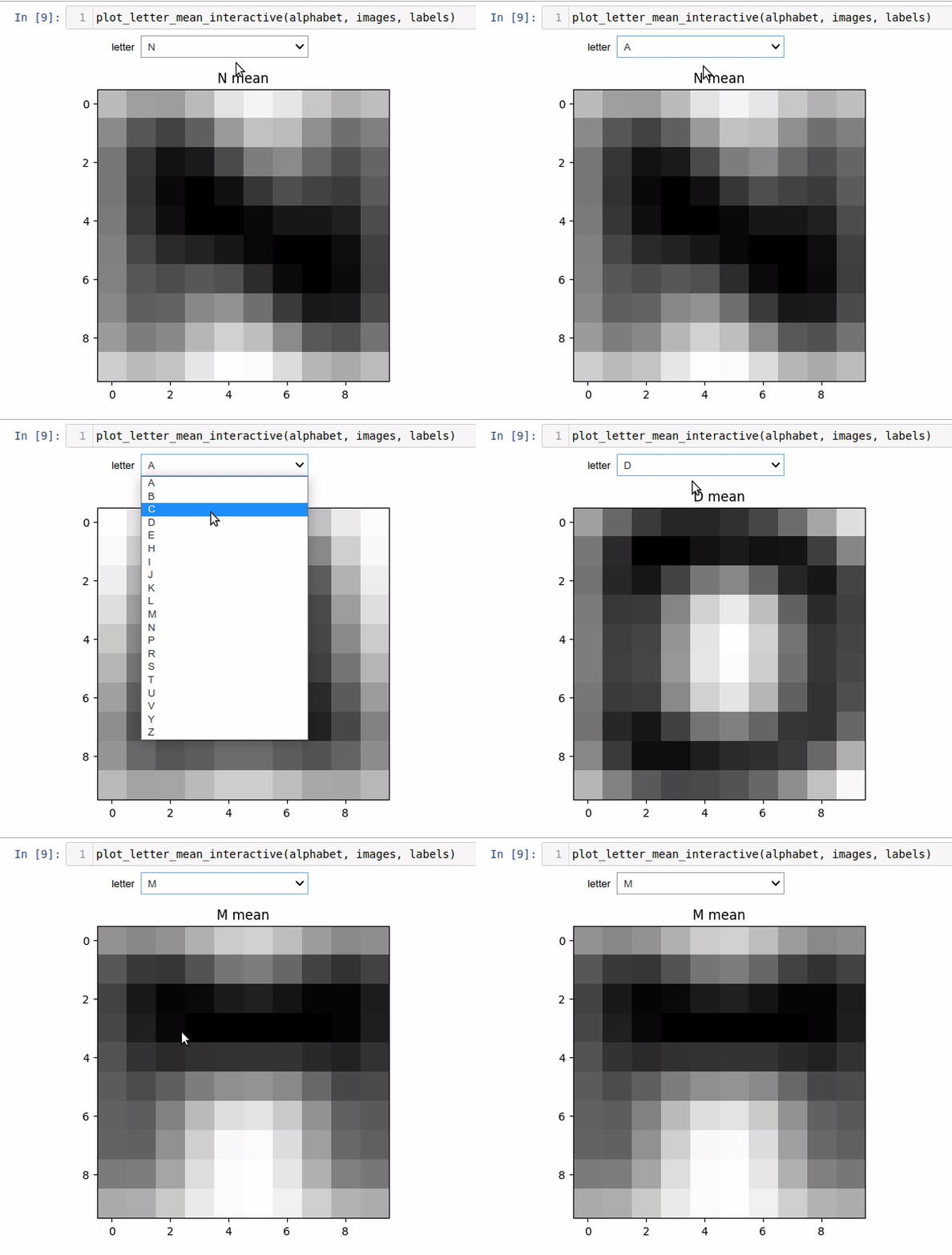
after importing matplotlib. - For a given letter, compute its mean image. This means taking all images in the dataset displaying that letter, and making pixel-wise mean. Use your name initials (if present in the dataset) and save them as
initial1_mean.pngandinitial2_mean.png(use any letter if any of your initials is not present in the dataset). Round the mean image to integers and return it in theuint8type.
- hint: Image generation is already prepared in
basics.ipynb - For the purpose of mean image calculation, complete the function
compute_letter_mean:letter_mean = compute_letter_mean(letter_char, alphabet, images, labels)
whereletter_charis a character (e.g. 'A', 'B', 'C') representing the letter whose mean we want to compute,alphabet,imagesandlabelsare loaded from the provided data, andletter_meanis the resulting mean image.
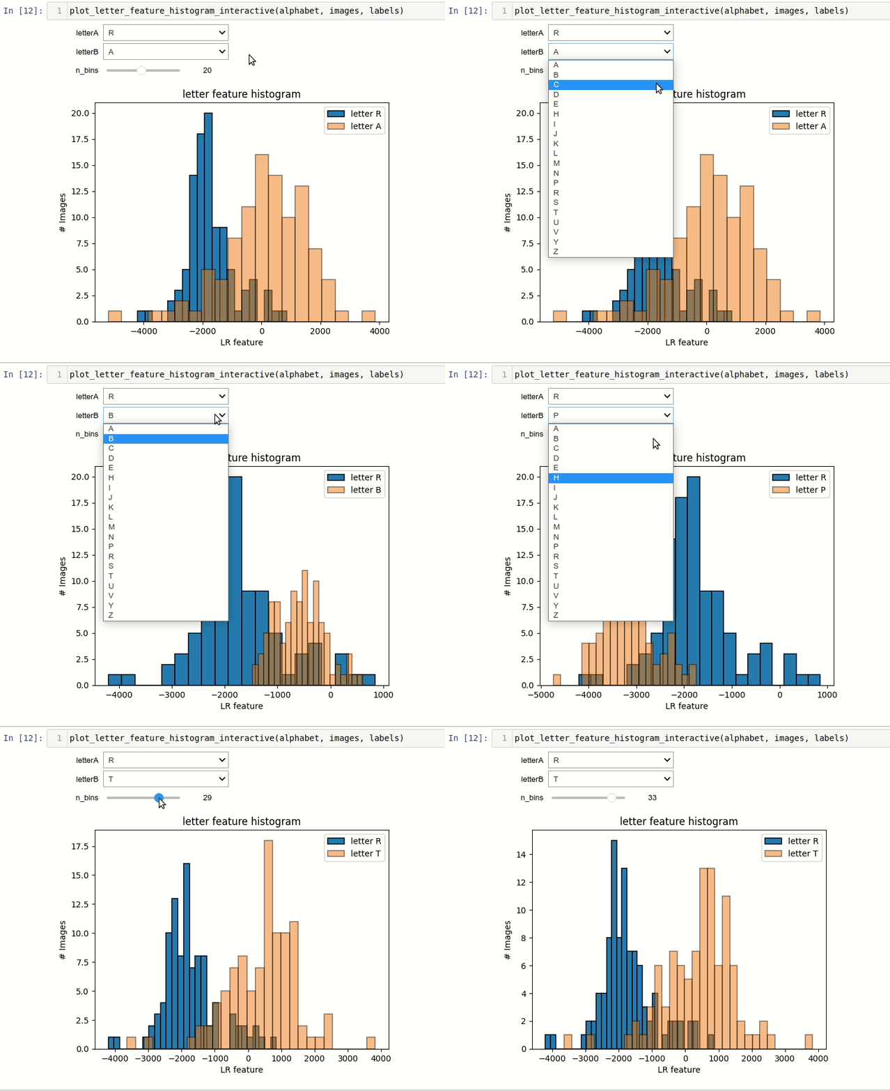
- Compute features (from images) for all occurrences of a given letter. For a single image, it is an image feature x - a single number characterizing an image. It is defined as
x = sum of pixel values in the left half of image - sum of pixel values in the right half of image
warning: The images are stored in unsigned type (uint8), make sure to convert the values to suitable signed type before doing the subtraction. E.g.np.int32(sum_left) - np.int32(sum_right).
Complete a function for the features computation:lr_features = compute_lr_features(letter_char, alphabet, images, labels)
whereletter_charis a character representing the letter whose feature histogram we want to compute,alphabet,imagesandlabelsare loaded from the provided data, andlr_featuresis the resulting vector of features for a given letter.- For reference the following feature vector was computed for a letter A
>> compute_lr_features('A', alphabet, images, labels)
array([  120  1223  -144  -161   197 -2921  -998  -944  -120  -304  -884 -1461
       -1233  1444  1705  1332   881   212    92   319 -3104 -2829   255     1
       -1763  2230  1916  -335  -257 -3568 -5204 -1144  -641   525   182  -768
        -844  1536  1139   522   495   353  -251  1345   439  1114 -2087  -107
        -563  1491 -1935 -1640  1979  2215   906  1726  1332   365   825  2776
        1282   708  1010   429  1141  1145  1896     7  -642  -657    36   368
        1079    79  -483   327  -135   888  2270  2211  3860  1248  1371  -857
         100  -134  -946  1954  1979 -1575  -837  1363   803   546 -1916 -1808
         370  -435  -363   497])
- Plot feature histograms of your initials into one figure to compare them and save the figure as
initials_histograms.png.- Code for plotting histograms already prepared for you as
plot_letter_feature_histogram(features_1, features_2, letters)
