Table of Contents
Image retrieval
In this lab we will implement a system to perform image retrieval from large databases. We will use the Bag-of-Word (BoW) approach to construct the image representation and use an inverted-file to perform the search efficiently. In this way, we will obtain an initial ranking of the database images. The ranking is done according to their relevance to the query as this is estimated with the BoW similarity. As a second step, we will perform fast spatial verification on a short-list of top-ranked images. This will allow use to estimate the geometric transformation between each top-ranked image and the query image, but also to find inlier correspondences. The number of inliers will be used to re-rank the short-list. Spatially verified images will be used to form an enriched query that will be used to perform query expansion.
1. BoW Image Representation. TF-IDF Weighting
Images are initially represented by a set of local descriptors extracted from normalized image patches. The BoW model relies on vector quantization in the space of local descriptors. Quantization is achieved by performing clustering on a large set of local descriptors. The resulting set of clusters, and the corresponding centroids, forms a visual vocabulary, where each cluster corresponds to a visual word. A visual word can be seen as a representative image patch that occurs often. A local descriptor is quantized by assigning it to the nearest centroid / visual word. The BoW approach represents an image by the set of visual words that appear in it, in the same way that a document is represent by the words that appear in it in natural language processing.
To perform vector quantization, we will implement K-means, which is a well known and commonly used clustering approach.
Vector Quantization - K-means
K-means should already be known from the Pattern Recognition course:
- Input: set of vectors, $k$
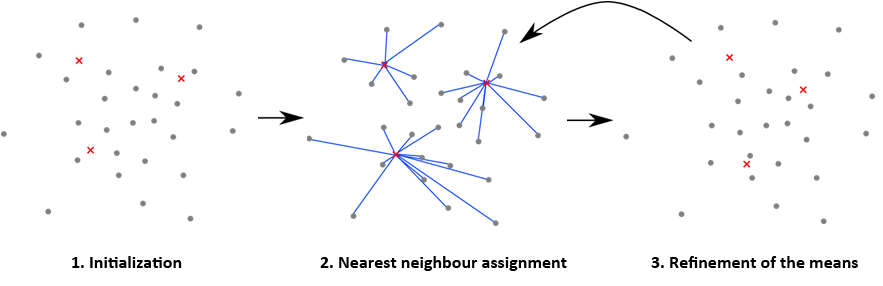
- Initialization: Choose an initial set of $k$ clusters centroids (the red crosses in the image). Random points can be chosen from the set of descriptors, but more sophisticated methods exist too.
- Assign each point to their nearest centroid
- Update each centroid to be equal to the center of gravity (mean) of the points assigned to it. In the case that a centroid has no assigned points, the centroid need to be updated to a new point.
Repeat steps 2 and 3 until the assignments in step 2 do not change, or until the change of the point-to-centroid distances decreases below some threshold.
Implement k-means:
- Write a function
nearest(centroids, data), which finds the nearest vector from the set of centroids (matrix with size KxD, where K is the number of centroids and D is the dimension of the descriptor space) for each row vector in matrix data (with size NxD, where N is the number of points). The output of this function is indices idxs (vector of length N) of the nearest centroids and distances dists (vector of length N) to the nearest centroid. - Write a function [centroids, err]=
kmeans(K, data), which performs K means on the vector set data and returns err as the sum of distances between data points and centroids they are assigned to.
We prepared the data for you (in the test archive at the bottom of this assignment) to make this assignment a little bit easier. (So the next paragraph is just to put things into a context. You don't have to do these steps in first assignment.).
In order to represent images by sets of visual words the following steps need to be performed:
- use the
detect_and_describefunction to extract image local descriptors using the same setting for all images and choosing parameters such that there is ca. 2000-3000 descriptors per image on average. - then we apply
kmeansfunction to all descriptors to obtain e.g. 5000 clusters. The cluster centers – vectors in descriptor space – and their indices are used as visual words for the image representation. - to find the visual words per image, we assign a visual word index to each local descriptor using the
nearestfunction and we store the vector of visual words indices representing the image. Similarly, we store information about geometry with parameters of frame [x;y;a11;a12;a21;a22].
Inverted file
After the previous step, every image is represented by a vector of visual word ids. We construct the BoW vector per image by counting the number of occurrences per visual word. Image similarity between two images is computed by the cosine similarity of the BoW vectors as:
<latex>\displaystyle\mathrm{score}(\mathbf{x},\mathbf{y}) = \cos{\varphi} = \frac{\mathbf{x}\cdot \mathbf{y}}{\|\mathbf{x}\|\|\mathbf{y}\|} = \frac{1}{\|\mathbf{x}\|\|\mathbf{y}\|}\sum_{i=1}^D x_i y_i</latex>
We can take advantage of the fact that a part of the similarity can be computed ahead and L2 normalize the vectors (L2 norm equal to 1). After that, the similarity can be computed as a simple dot product of two vectors.
The visual vocabulary can be very big, often with a few thousands or even millions of words. To simplify the similarity estimation between such long and sparse vectors, the so called inverted file is used. Inverted file is a structure, which for each visual word (A, B, C, D in the picture) contains a list of images <latex>\alpha</latex>,<latex>\beta</latex>,<latex>\gamma</latex> in which the word appears together with the number of occurrences.
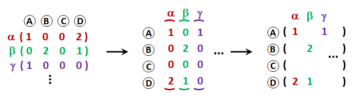
We will represent the database as a sparse matrix. A sparse matrix is a structure for the memory-efficient representation of huge matrices where most of the entries are zeros. We will use scipy implementation ( see scipy documentation for details). Our inverted file will be a 2D sparse matrix, where columns are images, and rows are visual words. For instance, the third row of the matrix will contain the number of occurrences of the third word in all images. We will L2 normalize each vector (i.e., divide by square root of the sum of squared number of occurrences). The vector that corresponds to each column of the matrix should have unit L2 norm.
- Implement a function
create_db(vw, num_words), which builds the inverted file DB in the form described above (sparse matrix NxM, where N=num_wordsis number of visual words in the vocabulary and M is the number of images. Argument vw is a np.ndarray of objects (object here is another np.ndarray), where each array contains the list of visual words per database image. Note: the sparse matrix should include the L2 normalized vectors. (For the sparse matrix, use the scipy function csr_matrix).
TF-IDF weighting
In real images, visual words tend to appear with different frequencies. Similar to words in the text domain, some words are more frequent than others. The number of visual words in one image is changing depending on the scene's complexity and the detector. To deal with these differences, we have to introduce a suitable weighting of visual words. One weighting scheme, widely used also in text analysis and document retrieval, is called TF-IDF (term frequency–inverse document frequency). Weight of each word $i$ in the image $j$ consists of two values:
$$ \mathrm{tf_{i,j}} = \frac{n_{i,j}}{\sum_k n_{k,j}},$$
where $n_{i,j}$ is the number of occurences of word $i$ in image $j$; and
$$ \mathrm{idf_{i}} = \log \frac{|D|}{|\{d: t_{i} \in d\}|},$$
where $|D|$ is the number of documents and $|\{d: t_{i} \in d\}|$ is the number of documents containing visual word $i$. For words that are not present in any image, <latex>\mathrm{idf_{i}}=0</latex>. The resulting weight is:
$$ \mathrm{(tf\mbox{-}idf)_{i,j}} = \mathrm{tf_{i,j}} \cdotp \mathrm{idf_{i}}$$
Note: the TF term is similar to the number of visual word occurrences we were using earlier (“inverted file” section) but differs in the existence of the denominator. The denominator has the same value for all vector elements of a particular image and, therefore, does not play any role due to the L2 normalization of the final vector (a constant multiplier is canceled out).
We need two functions
- a function
get_idf(vw, num_words), which computes the IDF of all words based on the lists of words in all documents. The result will be anum_words$\times$1 matrix. - adjust a function
create_dbto functioncreate_db_tfidf(vw, num_words, idf), which instead of word occurrences uses TF-IDF weighting (frequencies of each word multiplied by the IDF of the word). Normalize the resulting vectors to have unit L2 norm ($ \frac{1}{||x||}$ part of cosine similarity).
Image ranking according to similarity with query image
Thanks to the inverted file, we can rank images according to their similarity to the query. The query is defined by a bounding box in the query image around the object of interest. Only the local features with their center inside the bounding box are used to form the query representation. The visual words of the corresponding local descriptors are used to represent the query. Compute the BoW vector for the query and multiply it with the corresponding columns of the inverted file, matrix DB. The result is a similarity vector between the query and database images. (You don't have to create visual words selection on your own for now. It is mentioned to show context).
- write a function
query(DB, q, idf), which computes similarity of the query q - list of visual words and images in the inverted file DB. Parameter idf are IDF weights of all visual words. The result of this function is an array score with similarities ordered in descending order and img_ids, indices of images in descending order according to similarities.
What you should upload?
Upload file image_search.py with the before mentioned implemented methods.
Testing
To test your code, you can use a jupyter notebook test.ipynb in assignment_4_5_indexing_template. Data can be found here tfidf_test.zip. The notebook is also provided with expected results in commentaries. Feel free to use function get_A_matrix_from_geom in spatial_verification.py which returns geometry arranged into affine matrix.
2. Fast Spatial Verification. Query Expansion.
An initial ranking of the database images is obtained according to the BoW similarity (first of the lab). In this part, we will apply spatial verification on a short-list of top ranked images and re-rank them according to the number of inliers. Optionally, we will use the spatially verified images to perform query expansion.
Spatial Verification
After ordering according to tf-idf, we get a short-list of the K top-ranked images (also called relevant images in the following). We will apply spatial verification on this list of top-ranked images. Spatial verification (RANSAC-like process, but deterministic) takes tentative correspondences as input. Local features in the same visual word form a correspondence. If M and N are the number of features with the same particular visual word in the query image and a database image, respectively, then, this visual word gives rise to MxN tentative correspondences (Cartesian product of the feature sets). At most min(N,M) out of these are true correspondences. We will set two limits. Firstly, the maximum number of correspondences per visual word (max_MxN), and, secondly, the maximum number of tentative correspondence per image pair (max_tc). Moreover, we will prefer the visual words with smaller product MxN. In summary, to compute the tentative correspondences, the following process is followed: 1) sort common visual words w.r.t. MxN, 2) keep adding tentative correspondences in ascending order of MxN until a termination condition is met (either MxN goes beyond max_MxN or the number of correspondences goes beyond max_tc). A tentative correspondence is defined as a pair of indices; the indices are for the list of visual words per image (query and database image) indicating which features are in correspondence.
- Write a function
get_tentative_correspondencies(query_vw, vw, relevant_idxs, max_tc, max_MxN), which computes tentative correspondences. Correspondences are stored in an np.ndarray of objects (arrays). The k-th array will hold an array of Tk tentative correspondences between query and the k-th relevant image, as an array of storing pairs of indices into query_vw and vw, respectively. The input is a vector of visual words query_vw in the query image; array of arrays vw with arrays of visual words in images in the database; array of size K relevant of indices of relevant images. Finally, max_tc and max_MxN defines termination criteria.
Our local features are represented by affine frames. For this reason, we choose affine transformation as the geometric model for spatial verification which allows us to generate a transformation hypothesis from a single tentative correspondence. The hypothesis form a single correspondence is the affine transform that transforms one frame to the other. It is not necessary to use sampling, which results in speed benefits. We can verify all hypotheses (one for each tentative correspondence) and save the best one. The number of inliers will be the new score, which we will use for the re-ranking of the relevant images. The true geometric transformation between the query and the database image is not necessarily affine. For planar objects it is good as a local approximation of perspective transformation.
- Write a function
ransac_affine(q_geom, geometries, correspondencies, relevant, inlier_threshold), which estimates the number of inliers and the best hypothesis A of transformation from query to database image. Input is an array q_geom (Qx6, where Q is the number of words in the query) of geometries (affine frames [x;y;a11;a12;a21;a22]) of query visual words; array of objects geometries with geometries of images from the database; array of objects corrs and a list of relevant images relevant as in the previous function. The function returns an array scores (of size Kx1) with the numbers of inliers and a matrix of transformations A (matrix Kx3x3) between query and database image. Inlier_threshold is a maximal Euclidean distance of the reprojected points.
- Join the spatial verification with tf-idf voting into one function
query_spatial_verification(query_visual_words, query_geometry, bbox, visual_words, geometries, DB, idf, params), which orders images from database according to number of inliers. The result will be output of functionransac_affinejoined with output of functionquery(first part of the lab) where query score is higher than parameter minimum_score. Only top K (parameter max_spatial) images will be processed by spatial verification. Score of relevant images will be added to score from functionquery. img_ids will be the ordered list of image indices according to the new score. Return also ordered inliers_counts and corresponding transformation matrices. Input parameters will be the same as described above, with one expception – parameters query_visual_words and q_geom will contain all visual words from the query and parameter bbox (a bounding box in form [xmin, ymin, xmax, ymax]) which will be used for visual word selection. Parameter params will contain the union of parameters for functionsransac_affineandget_tentative_correspondencies, maximal number of images for spatial verification (maximal length of parameter relevant) will be set in field max_spatial.
Query Expansion
(optional task for 2 bonus points)
We consider the images that have high enough scores with spatial verification (for instance, at least 10 inliers) to be spatially verified. For each verified database image, the centers of local features are projected by transformation A-1 and features which are projected inside the query bounding box are added to the expanded query. The local features of the original query are added to the expanded query too. It is a good idea to constrain the total number of local features in the expanded query. We will restrict the number of local features in the expanded query to be less than max_qe_keypoints, simply by skipping the rest of the spatially verified images. It is also desirable to choose local features which add useful information. We will skip visual words with many (more than 100) occurrences in a particular database image; the associated local features should not be included in the expanded query.
- add query expansion to the function
query_spatial_verification. Query expansion will be used if the parameter use_query_expansion is True. The other parameters are the same.
Testing
To test your code, you can use a jupyter notebook (where you can also see a reference solution). In template you are also provided with utils.py where you can find tools for results visualization. Copy the file with mpvdb_haff2.mat database, unpack archive with images and put it into data directory in template.
Upload your image_search.py and spatial_verification.py in a single archive into 06_spatial task. Do not upload utils.py.
For this task, there is no auto evaluation; results will be checked by hand!
3. Image Retrieval in Big Databases
We will use a set of 1499 images as a database to perform image retrieval. It consists of 225 images from your colleagues from a previous year, 73 images of Pokemons, 506 images from dataset ukbench and 695 images from the dataset Oxford Buildings. We have computed features with detector sshessian with Baumberg iteration (haff2, returns affine covariant points). We have estimated dominant orientation and computed SIFT descriptors. We have computed a visual vocabulary of 50000 cluster centers from SIFT descriptors and we have assigned all descriptions to visual words. You can find the data in file mpvdb50k_haff2.mat, where array of arrays with the visual words per image is stored in variable VW, array of arrays with geometries per image in variable GEOM and names of the images in the variable NAMES. Cluster centroids are stored in file mpvcx50k_haff2.mat in variable CX. Compressed images are in file mpvimgs1499.zip. Local descriptors of these images are in file mpvdesc_haff2.mat, stored as array of arrays DESC. Each of these arrays has elements of type UINT8 and has size 128xNi, where Ni is number of points in ith image.
Choose 7 images:
- 3 from Oxford Buildings dataset
- 2 Pokemons: X=(your index in class MPV)-1, your images are those with index from (2*X) to (2*X+1).
- 2 from dataset ukbench.
On each of these 7 image chose a rectangle to define the object to search for and the query region. Use only local features, which have centers inside the bounding box (including boundary). With function query_spatial_verification query the database and find results.
Prepare a jupyter notebook where you show your results using
utils.query_and_visu(q_id, visual_words, geometries, bbox_xyxy, DB, idf, options.copy(), img_names, figsize=(7, 7)) for visualization (as done in jupyter notebook in previous task).
Then you transform your notebook into file results.html using
jupyter nbconvert –to html my_results_on_big_db.ipynb –ExecutePreprocessor.timeout=60 –EmbedImagesPreprocessor.resize=small –output results.html
Then put results.html into archive and upload file into 07_big_db.
figsize=(7, 7) in visualisation, shouldn't be a problem.