Table of Contents
List of projects
It is possible to choose your topic (which is also preferred), as difficult as you see fit. Rather than the complexity of the topic, the way how the student implemented the problem in Matlab will be evaluated (see criteria HERE). Please look at the projects as a chance to practice your habits in Matlab ![]()
Project example
Animation of electromagnetic field
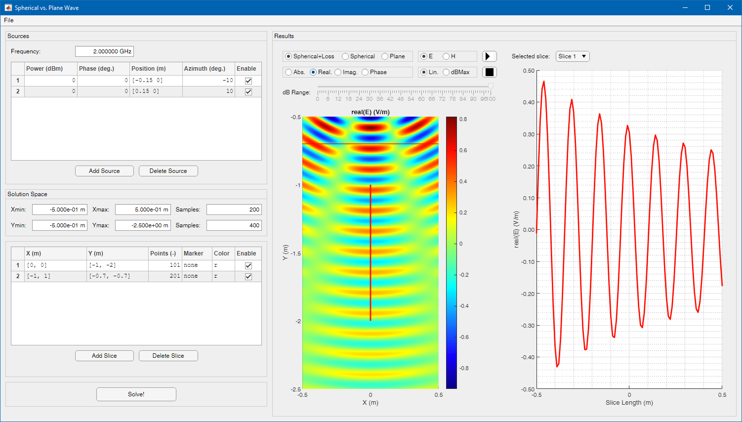 This project allows you to compare and animate the electromagnetic field emitted by point sources, or plane waves. Field sources can be entered any amount. Each source is defined by radiated power, initial phase, position and azimuth. The azimuth is only used to replace the point source by a plane wave that radiates from the specified azimuth. You can also select solution space in which the field will be calculated and you can define slices through this space. Fields along slices can be analyzed in separate graph. The displayed field is in the XY plane for Z = const. All considered point sources are also in this plane. All sources have the same polarization. The project allows to consider three approaches to field generation: point source with consideration of field attenuation in space according to 1/R^2, point sources without field drop along the distance and plane wave. The main.m file is running in MATLAB 2020b or later. The project serves as an example of an above-standard semester project, which would be evaluated by the full number of points.
Project proposals
For most projects, at the end of the description in parentheses is the abbreviation of the name of the teacher who created the assignment and is responsible for the project. Consult this project with this person on an ongoing basis - the description of the project is not considered to be the description below. Still, only the specific form agreed with the teacher!
| Abbrevation | Name | |
|---|---|---|
| MČ | doc. Ing. Miloslav Čapek, Ph.D. | miloslav.capek@fel.cvut.cz |
| VA | Ing. Viktor Adler, Ph.D. | adlervik@fel.cvut.cz |
| VL | Ing. Vít Losenický | losenvit@fel.cvut.cz |
| MM | Ing. Michal Mašek | michal.masek@fel.cvut.cz |
| RK | Ing. Rostislav Karásek | karasros@fel.cvut.cz |
| LJ | doc. Ing. Lukáš Jelínek, Ph.D. | lukas.jelinek@fel.cvut.cz |
| PK | Ing. Petr Kadlec, Ph.D. | kadlecp@feec.vutbr.cz |
| MP | Ing. Milan Příhoda, Ph.D. | milan.prihoda@cst.com |
| TK | Ing. Tomáš Kořínek, Ph.D. | tomas.korinek@fel.cvut.cz |
Apps
- Any custom theme. However, it is necessary to consult the topic first and make an agreement on the content of the project.
- Reference converter and parser (MC)
- Propose a scheme for automate conversion of DOI (unique identifiers of scientific papers) to LaTeX bib format. Project will utilize web API and remote control of web converter. Downloaded entries will be parsed and written into bib file.
- Mortality statistics of the population of the Czech Republic (VA)
- Create an interactive browser of mortality tables from the years 1920 - 2018 from the Czech Statistical Office. The tool can take many forms; you can display, for example, the number of deaths at a particular age depending on the year, allow comparisons between men and women, display the population of a given age, the relative probability of death at a certain age, the frequency of deaths depending on the season, etc.
- Creating a simple application that will do anything (text editor, image editing, calculator, audio editing, …), but will support history and its editing. (VA)
- The application should have a “Back” and “Forward” button and a command history editor that allows you to delete and move items in the history and then execute the entire history.
- Interactive editor of RLC circuits, including the creation of jumpers and the generation of the matrix form of the resulting connection (VA)
- Creating and displaying a Smith diagram (VA)
- The task is to create a function that displays parametric circles in the polar axes (
polaraxesfunction) as is common with Smith's diagram (wiki). Only a few circles are enough for the most important relative values of reactances (eg 0.1, 0.3, 0.5, 1, 3, 5, 10, …). The function must also be able to plot the image coefficient in the Smith diagram thus created, which will be one of the inputs of the function in the form of a column vector. The next of the inputs will be frequency points. There must be some controls in the graph window (setting lines, markers, switching impedance/admittance diagram, etc.).
- Random walk of several agents in a limited area (MČ)
- At the beginning, consider agents randomly distributed in a given area (“drunks”), who move around the delimited area (“park”) randomly. Generate their motion, display it, analyze the average values (speed, position) and develop techniques for keeping agents inside areas (reflective wall, absorption wall, …).
- Type reader/writer for 1D and 2D geometry for * .dxf, * .svg and * .eps (PK)
- Processing of *.gpx files with data from GPS receivers(VA)
- Evaluation of route length, elevation, speed, calories burned, route display in maps, … it is up to you.
- To read data from *.gpx files use the function loadgpx.m.
- Display the route on the map using the
geoplotfunction, resp. classGeographicAxes(functiongeoaxes). - To compute the actual distance between points on Earth you can utilize https://en.wikipedia.org/wiki/Haversine_formula.
- Test data: praguerunning.zip.
- GPX format documentation: https://topografix.com/gpx.asp.
- Evaluation of signal parameters (VA)
- Analyze whatever time-dependent signal you like (electrocardiogram - EKG, sound, music, temperature, sea-level, …)
- Load the signal from file, show signal in a graph and analyze signal's basic parameters.
- Control of any device/toy/kit from Matlab (VA)
- Whatever comes to your mind. But you must have your own controlled device. E.g., you can write a GUI to control a device on the popular Arduino platform because Matlab natively allows you to send and receive messages over a serial line (function serialport).
- This is mainly a final project for the MATLAB course, i.e., the project will be evaluated from the point of view of Matlab and not, for example, from the Arduino language. From this point of view, Arduino should only work as an executor of orders, and as much of the project as possible should be handled in Matlab.
- Use the class Serial to receive and send messages via the serial line to Arduino.
- Simulation of the motion of bodies in the solar system (VA)
- Calculation and visualization of the trajectory of bodies of the solar system from the elements of the path of bodies. It is not absolutely necessary that the position of the planets exactly corresponds to the selected date. But try to observe the parameters of elliptical orbits and orbits of planets. Represent the planets somehow nicely and allow you to change the speed of the motion simulation. Required data: http://ssd.jpl.nasa.gov/?planet_pos
- Möbius net (MČ)
- Oscilloscope in Matlab (VA)
- Implement a simple oscilloscope that will display signals from the sound card input. Use class
audiorecorder( example). - The oscilloscope should be reasonably usable, so to display periodic signals, it is necessary to ensure the adjustment of the vertical and horizontal scale and the triggering of the time base to the edge of the signal. The trigger level should also be adjustable.
- Try an effective implementation, where the image is redrawn, for example, a maximum of ten times per second, even if it would be more common for some timebase settings.
- Vector meter of impedance and transmission of circuits using a sound card (VA)
- An unknown circuit will be excited by the output of the sound card, and the output signal will be recorded by the input of the sound card. By analyzing the signals, you evaluate what impedance or circuit transmission has been connected. It is necessary to solve incl. calibration. The program can be designed, for example, especially for measuring audio amplifiers, incl. evaluation of THD distortion, etc. Use class
audiorecorder( example).
- Matlab console (tokenizer) (MČ)
- Develop a simple GUI that allows you to enter (load) a text string. Then process it inside the program, which will then execute the specified commands.
- Rendering and animation of the Lorenz attractor (MČ)
- Create an application that allows you to load a base object and then apply the specified symmetric operations to it and create an overall structure. (MM)
- Statistical analysis (VA)
- From any sufficiently representative sample of any data (wind direction, temperature, sewage flow, lighting intensity, number of shop visitors, animal population, …) calculate and display statistical parameters (distribution function, standard deviation, mean, median, quartiles,. ..). In the application, enable data loading and interactive change of displayed parameters.
- Splitwise in MATLAB (VL)
- Create an app that allows you to create a shared payment bill for a group of people (e.g., for a trip together). Design an algorithm to optimize the number of payments that must be made to settle the billing (you can be inspired here).
- *.gpx file editor (VL)
- Create an application that allows you to modify *.gpx files (modify the recorded route: trim the record, change the position of the recorded points, …)
- Orienteering run analyzer (VL)
- It implements an application that allows you to analyze and compare the running of several runners (you can be inspired by 3Drerun).
- Allow to load and calibrate the scanned/photographed map, set the playback speed, the size of the tail behind the runner, time synchronization, …
Audio / Video
- Creating a panoramic photo (VA)
- Create an application where it is possible to: load individual figures of a panorama scene, set figure's parameters if necessary, create a panorama from figures, set proper crop of final panorama, save figure as standalone file. Workflow can be modified as needed.
- Tuner of musical instruments (VA)
- Vectorization of bitmap (scanned) graphs (VA)
Games
- Arkanoid (VL)
- Quoridor (MČ)
- Implement a game board, enter tiles and control a piece, try to find a primitive game algorithm.
- MiniMetro (MM)
- Hnefatafl or another version of the Old Norse board game wiki (MM)
- Any game using the transportation network system, e.g. Pocket Trains (MM)
- suitable to work with OOP, timers
- Sokoban (VL)
- suitable to work with OOP, timers
- Display and automatic solution of a Rubik's cube (VA)
- Billiard game (VL)
- Worms (MM)
- Can't Stop game (MM)
- Hill Climb Racer (VL)
- Tower defense (MM)
- Space Invaders (VL)
- Create a single-player UI for the board game Cartographers EN info. Background materials would be provided. (MM)
- Create a game that uses a hexagonal playground, see Implementation notes (VL)
- Lunar lander game remake (VL)
- Atomic Bomberman (VL)
Numerical calculations
- External ballistics (VA)
- Display the trajectory of the projectile and calculate the necessary correction of the riflescope to hit the target for a specific distance, elevation, ammunition, wind speed, position on Earth, …
- Calculation and display of the Foucault pendulum at various points on the planet (VA)
- Thomson problem (LJ)
- Distribution of N equal charges on the surface of the sphere so that they have an overall minimum potential electrostatic energy.
- Finding the intersections of general curves given by an analytical formula (PK - VUT)
- Numerically, without the use of a symbolic toolbox.
- For a general body (given by boundary points), find such a center describing the sphere so that this sphere is the smallest possible. Then move the body so that it is inside this sphere, which is centered in the center of the Cartesian coordinate system. Display the body before and after moving it together with the wrapping ball. (MČ)
- Tool for displaying and calculating EM tasks using the method of mirroring + visualization (MČ)
- A generalized solution of loop currents / nodal voltages (MČ)
- Calculation of geometric and physical center of gravity of an object/system of objects (MČ)
- Multicriteria optimization (PSO / GA), including a display of the resulting Pareto front (MČ)
- Nelder-Mead optimization (MČ)
- Create a simplified algorithm of simplex optimization (space is searched using simplex with the help of its successive transformations.
- Spline interpolation of the specified name using curve extremes (MČ)
- The program writes the entered text string to the window (figure), then using the
ginputfunction, the vertices of the spline curves will be entered. The task will be to properly parameterize these curves so that the original text is reconstructed as best as possible.
- Excitation of waves on a 2D surface (solution of a wave equation using FDTD) + visualization (LJ, MČ)
- Swarm optimization (MČ)
- Study the swarm optimization algorithm (PSO) and try to implement it for the case of one-criteria, multidimensional optimization.
- 1D 3rd-degree interpolation (cubic) (MČ)
- Finding the minimum of a function using a gradient algorithm and its modification to find the global minimum in the presence of a series of local minima (e.g. function or f (x) = 1 - cos (x) + x ^ 2 / a ^ 2 on the interval x = [-a, a]) - Monte Carlo, stochastic algorithms.
- Simplified Ray Tracing method for studying beam propagation (MČ)
- Create a simple tool to calculate the charge distribution on a surface (MČ)
- It will be possible to create the surface using a simple GUI; the calculation of the charge distribution can be based, for example, on the knowledge of Coulomb's law and superposition (the calculation will be performed iteratively). The result will be a visualization of the current position of all charges (the number and initial position will be entered by the user), as well as the direction of their movement.
- There is a simple example in 1D.
- Fluid Dynamics (VL)
- Creation and solution of a maze (VL)
- Circuit analyser (MC)
- Implement formulas (they will be provided) for analysis of arbitrary circuit represented by interconnected N-ports.
Other
- Virtual circuit analyzer (GUI). (MP)
- The program will be used to estimate measurement errors using a circuit analyzer. The program will contain a realistic model of the device with adjustable parameters; calibration techniques, and visualization of results and deviations [Michael Hiebel, Fundamentals of Vector Network Analysis, 3rd ed. (Rohde & Schwartz, Munich, 2008). 420 pp. [ISBN: 978-3-939837-06-0]
- Extraction of material properties (TK)
- Based on the knowledge of S-parameters obtained by simulations of known materials inserted into the waveguide part in CST MWS, design and implement a method for extracting material parameters. The method developed must include corrections about the dimensions of the materials and the reference planes of measurement. Verify the method of extraction of material parameters on real measurements using VNA.
- Approximation of the elevation profile of refractivity in the troposphere (PP)
- There is a value of refractivity measured at 19 different heights above the ground. Approximate this data by polynomial 1.-4. order according to the user's choice and graphically display, including the measured points. Graphically display the first derivative of the function and highlight the areas with the possibility of occurrence of a waveguide channel, i.e., when the gradient of the height profile of refractivity is less than -157 N/km. (Note: Refractivity is the recalculated refractive index of the atmosphere. It is a function of temperature, pressure, and humidity. The distribution of refractivity in the troposphere fundamentally affects the propagation of radio signals due to refraction.)
- A moving average (PP)
- There is a non-equidistant time series of received signal levels measured by the mobile terminal. With a known speed of the terminal and the frequency of the signal, perform a conversion depending on the dependence of the received level on the distance in the wavelength scale. Apply moving average signal filtering and display in the same graph the original and several filtered waveforms from different sizes of the moving window (the interval in which we average) according to the user's input. (Note: This is a classic method of separating rapid leaks caused by multipath wave/signal propagation.)
Projects you CAN'T choose from! (temporarily discarded)
- Creation and representation of Platonic solids (VL)
- Implement a simple program that allows you to create and display Platonic solids.
- Matlab Planetarium (VA)
- Display of the star sky at any time and from any position on Earth. But it's not too easy. The position of objects in the sky is given by the current rotation of the Earth relative to the stellar sphere and is governed by the so-called stellar time. From this, the position of the azimuth https://en.wikipedia.org/wiki/Spring_point> of a spring point can be calculated. Furthermore, it is necessary to calculate the elevation of stars due to the tilt of the Earth's axis, see. also astronomy.cz.
- You can also implement a map of the sky by directly selecting the specific RA and DE coordinates of what the field of view and part of the sky should be displayed. It is advisable to be able to interactively set how faint stars still appear and be able to move with the viewport across the sky.
- Audio files editor (VA)
- Ability to load an audio file, view its progress, edit audio (crop, volume, equalization, a few effects, …), save.
- Video files editor (VA)
- Possibility to load a video file, display the timeline, edit the video (cut, brightness, contrast, …), save to individual images, and to the video. Choice of output format, image size (interpolation), and quality.
- 2048 (VL)
- Flappy bird (VL)
- Fourier transform (MČ)
- Double integral integration with look-up-table algorithm (MČ)
- For the given double integral (it does not have a simple primitive function, numerical integration is required) and the data obtained from the multiphysics solver in the form of a table, design an integration procedure with interpolation in the table (look-up-table).
- Minimization using the nonlinear least-squares method (MČ)
- Study the least-squares method and its nonlinear variant and try to compare individual approaches in Matlab on selected examples.
- Calculation and display of spherical functions, their superposition, correlation with general spherical functions (MČ)
- Programming a simple “snake” game in Matlab (MM)
- Simplified piano in Matlab
- Generate the necessary piano tones in Matlab, then process the keyboard input (“keyboard”). Try to find a suitable signal envelope to eliminate the synthetic sound of the keys.
- Chess (MM)
- Draw a chessboard, incl. the correct description of the axes. Next, place pieces (eg pictures) on this chessboard. With these pieces, it will be possible to move according to the rules of chess.
- Photo editor (VA)
- Load, save, basic adjustments (brightness, contrast, saturation, crop, resampling, …), filters (sharpen, blur, …).
- Pong (VA)
- SUDOKU game, loading the puzzle from the file, user game, following the rules (VL)
- Hra Quarto (MČ)
- Find algorithms that detect the shortest path to victory, when the game has no solution (end of the game), or the move that will prolong the path the most.
- Space Impact Game (VA)
- A simple implementation of the game Space Impact known from older Nokia mobile phones
- Tetris (VA)
- Game of life (VL)
- Tic-tac-toe (with AI)(VL)
- Draughts (with AI)(VL)
- Battleship (VL)
- Try to formalize and implement a ship game in Matlab. Your opponent will be a computer that chooses positions pseudo-randomly (or pseudo-randomly with respect to the last successful hit).
- Visualization of 2D / 3D functions with user input
- Develop a program that will be able to visualize 2D / 3D vector functions. Use vectorization and quiver functions to render.
- Tool for extracting help and H1 lines from user-defined Matlab functions
- It is a project focused on reading text strings from specified files and their processing. Suitable for students with knowledge of LaTeX.
- Creating a mex library
- ADC (analog to digital signal converter) - sampling, quantization, visualization of general signal
- Gaussian elimination, Gaussian elimination with pivots + comparison with Matlab build-in function
- Correlation analysis (find a known signal, in a noisy received signal)
- Use of the accumulation method to enhance the repeat signal in the noise
- Mortgage calculator (FK)
- A solution to an equation of type f (x) = 0 using the interval division method and using Newton's method (MČ)
- Jacobi method (eg surface generation from the knowledge of the perimeter curve, or calculation of electrostatic potential - the core of the method is written) (MČ)
- Implementation of FIR digital filter in limited accuracy (PČ)
- Implementation of IIR digital filter in limited accuracy (PČ)
- Each set of linearly independent equations can be orthogonalized to find the orthonormal basis of the subspace that these equations generate.
- Optimization of RLC structure or filter with the possibility to select values of components from the standardized series E6 / E12 / E24 (VA)
- Vectorized 2D interpolation (VA)
- MSDN Library in Matlab (VA)
- Explore and try to use the MSDN Library for advanced graphics in Matlab
- Design of a calibration kit for measurement with a circuit analyzer (GUI). (MP)
- The program will be used to optimize the parameters of calibration standards according to specified criteria. The program will propose calibration standards for Multiline TRL measuring technology http://dx.doi.org/10.1109/22.85388
- Processing of measured data from the circuit analyzer (GUI).(MP)
- It is a project focused primarily on creating a graphical interface. From the measured parameters of the three samples, determine the propagation constant of a homogeneous transmission line of a given length. Design a graphical interface for visualizing the results of the calibration algorithm, see [V. Sokol, Jan Eichler, Marc Rütschlin: “Calibration of EM Simulator on Substrate Complex Permittivity”, ARFTG 83rd Microwave Measurement Conference, Tampa, 2014]. It is a cooperation with the results usable potentially in practice, a functional algorithm is available.
- Icon editor (VA)
- Painting icons with dimensions 16×16 px and their export for use in
uipushtoolfor creating your own menu.
- Connect Four (VL)