Table of Contents
Support Vector Machines (SVM) for Non-linear Classification
In the last lab, we have implemented the soft margin SVM algorithm. We have seen that in contrast to the Perceptron algorithm, the SVM can handle noisy training data (i.e. data which are in fact linearly separable, but due to errors in labels or measurements they are not). This is a very nice and important feature of a classifier, but can we handle somehow also data which are really linearly non-separable? Can we apply the same trick as was used in the Perceptron algorithm, i.e. the dimensionality lifting (aka straightening the feature space)?
In this lab, we will extend the SVM algorithm to the non-linear classification. We will use so called kernel trick, which enables us to use a linear classifier on linearly non-separable data by increasing the dimensionality of the feature space.
Given a fixed nonlinear feature space mapping $\phi(\mathbf{x})$, the kernel function is defined as follows $$ k(\mathbf{x}, \mathbf{x}') = \phi(\mathbf{x})^\top\phi(\mathbf{x}') $$
As we can see, the kernel is a symmetric function of its arguments, i.e. $k(\mathbf{x}, \mathbf{x}') = k(\mathbf{x}', \mathbf{x})$. The simplest kernel is obtained when $\phi(\mathbf{x})$ is the identity mapping $\phi(\mathbf{x}) = \mathbf{x}$ resulting in the linear kernel $$ k_L(\mathbf{x}, \mathbf{x}') = \mathbf{x}^\top\mathbf{x}'$$
Recall the classification function from the previous task $ f(\mathbf{x}) = \mathbf{w}^\top\mathbf{x} + b = \sum_{i=1}^m \alpha_i y_i \mathbf{x}_i^\top \mathbf{x} + b$ and the corresponding learning task:
The soft-margin SVM dual task $$ \vec{\alpha} = \arg\max_{\vec{\alpha}} \sum_{i=1}^{m} \alpha_i - \frac{1}{2} \sum_{i=1}^{m}\sum_{j=1}^{m}\alpha_i \alpha_j y_i y_j \mathbf{x}_i^\top\mathbf{x}_j, $$ subject to \begin{align} 0 \le \alpha_i & \le C,\quad i = 1, \dots, m \\ \sum_{i=1}^{m} \alpha_i y_i & = 0 \end{align}
Note that in both the learning task and the classification function the original data appear only in the form of a dot product ($\mathbf{x}^\top\mathbf{x}$). So, we could say that we were using the linear kernel SVM with the $k_L$ kernel.
Kernel trick (or kernel substitution)
The trick assumes that we have an algorithm where the input vectors $\mathbf{x}$ are used only in the form of a dot product and uses the idea of expressing a kernel as a dot product in the feature space, $\phi(\mathbf{x})^\top\phi(\mathbf{x}')$. By defining the mapping or the kernel we can then substitute it for the dot product.
The biggest advantage of using the kernel is that we do not even have to know the feature space mapping $\phi(\mathbf{x})$ explicitly. In fact it might even be a mapping to an infinite dimensional space! However not any symmetric function $k(x,x')$ is a kernel. The exact characterization is given by the Mercer's theorem: a symmetric function $k(\mathbf{x},\mathbf{x}')$ is a kernel if and only if for any $n>0$ for any points $\mathbf{x}_1, \dots \mathbf{x}_n$ the matrix $\mathbf{K}_{i,j} = k(\mathbf{x}_i,\mathbf{x}_j)$ is positive semidefinite: for all $\mathbf{\alpha} \in \mathbb{R}^n$ there holds $\mathbf{\alpha}^\top \mathbf{K} \mathbf{\alpha} \geq 0$.
Here are some commonly used kernels you will need for the assignment:
- Linear kernel:
$ k_L(\mathbf{x}, \mathbf{x}') = \mathbf{x}^\top\mathbf{x}' $
- Polynomial kernel of power $d$:
$ k_P(\mathbf{x}, \mathbf{x}') = ( 1 + \mathbf{x}^\top\mathbf{x}' )^d $
- Gaussian kernel (aka RBF kernel):
$ k_{RBF}(\mathbf{x}, \mathbf{x}') = e^{ \frac{ - \| \mathbf{x} - \mathbf{x}' \|^2_{2} }{2\sigma^2} } $
 Try to change parameter C and RBF kernel sigma to see how they influence the result.
To fulfil this assignment, you need to submit these files (all packed in a single .zip file) into the upload system:
answers.txt- answers to the Assignment Questionssvm2.ipynb- a script for data initialisation, calling of the implemented functions and plotting of their results (for your convenience, will not be checked)svm2.py- implementing the following functionsget_kernel- a function implementing various kernelsmy_kernel_svm- a function which implements the learning of the kernel svm classifierclassif_kernel_svm- a function which classifies given datacompute_kernel_test_error- a function computing mean error on test data from cross-validation
flower_rbf.png, flower_polynomial.png, ocr_polynomial_kernel_tst.png, ocr_svm_classif.png, mnist_tst_classif.png- images specified in the tasks
Use template of the assignment. When preparing a zip file for the upload system, do not include any directories, the files have to be in the zip file root.
Part 1: Kernel SVM
- Complete the function
get_kernel(Xi, Xj, options).
Given the input matrices $\mathbf{X}_i$ of size $n \times p$ and $\mathbf{X}_j$ of size $n \times q$, the function outputs the kernel matrix ($p \times q$), where $n$ denotes dimensionality of the features and $p,\ q$ denote the number of examples. The type of a kernel is specified in fieldoptions[“kernel”].
Hint 1: See the template and the introductory text above for the definition of expected kernel implementations.
Hint 2: The reason why we allow different dimensions $p$ and $q$ is, because this allows us to easily use this function also in classification.
X = np.array([[1, 2, 1, -1, -1, -2], [1, 1, 2, -1, -2, -1]])
y = np.array([1, 1, 1, -1, -1, -1])

K = get_kernel(X, X, {'kernel': 'linear'})
print(K)
# -> [[ 2  3  3 -2 -3 -3]
# ->  [ 3  5  4 -3 -4 -5]
# ->  [ 3  4  5 -3 -5 -4]
# ->  [-2 -3 -3  2  3  3]
# ->  [-3 -4 -5  3  5  4]
# ->  [-3 -5 -4  3  4  5]]
K = get_kernel(X, X, {'kernel': 'polynomial', 'd': 2})
print(K)
# -> [[ 9 16 16  1  4  4]
# ->  [16 36 25  4  9 16]
# ->  [16 25 36  4 16  9]
# ->  [ 1  4  4  9 16 16]
# ->  [ 4  9 16 16 36 25]
# ->  [ 4 16  9 16 25 36]]
K = get_kernel(X, X, {'kernel': 'rbf', 'sigma': 1.0})
np.set_printoptions(precision=4, suppress=True)
print(K)
np.set_printoptions()
# ->  [[1.     0.6065 0.6065 0.0183 0.0015 0.0015]
# ->   [0.6065 1.     0.3679 0.0015 0.0001 0.    ]
# ->   [0.6065 0.3679 1.     0.0015 0.     0.0001]
# ->   [0.0183 0.0015 0.0015 1.     0.6065 0.6065]
# ->   [0.0015 0.0001 0.     0.6065 1.     0.3679]
# ->   [0.0015 0.     0.0001 0.6065 0.3679 1.    ]]
- Complete the function
my_kernel_svm(X, y, C, options). This function solves the dual task of the soft margin SVM and uses the kernel specified inoptions[“kernel”]. The output of this function is a python dictmodelwhich contains support vectors (not just indices this time!), labels of support vectors, non-zero Lagrange multipliers $\alpha$, dictoptionscontaining the information about the kernel used, the bias term inmodel[“b”]and the function which will be used for classification inmodel[“fun”].
Hint: Use the functionget_kernelto compute the matrix $\mathbf{H}$ for QP task.
Hint: Use the providedcompute_biasfunction.
X = np.array([[1, 2, 1, -1, -1, -2], [1, 1, 2, -1, -2, -1]])
y = np.array([-1, 1, 1, 1, -1, -1])
C = float('inf');
options = {'verb': True,
           't_max': float('inf'),
           'kernel': 'rbf',
           'sigma': 0.01}

model = my_kernel_svm(X, y, C, options)
print(model)
# -> t=1, KKTviol=2.000000, tau=1.000000, tau_lb=0.000000, tau_ub=inf, Q_P=-1.000000
# -> t=2, KKTviol=2.000000, tau=1.000000, tau_lb=0.000000, tau_ub=inf, Q_P=-2.000000
# -> t=3, KKTviol=2.000000, tau=1.000000, tau_lb=0.000000, tau_ub=inf, Q_P=-3.000000
# -> {'sv': array([[ 1,  2,  1, -1, -1, -2],
# ->               [ 1,  1,  2, -1, -2, -1]]),
# ->  'y': array([-1,  1,  1,  1, -1, -1]),
# ->  'alpha': array([1., 1., 1., 1., 1., 1.]),
# ->  'options': {'verb': True,
# ->              't_max': inf,
# ->              'kernel': 'rbf',
# ->              'sigma': 0.01},
# ->  'b': 0.0,
# ->  'fun': <function classif_kernel_svm at 0x7fd4f1c56e18>}

- Complete the function
classif_kernel_svm(X, model).
The function applies a trained SVM classifier stored inmodelon the dataXand outputs their classification labels.
This function is important for drawing the separating hyperplane byplot_boundary(provided in the template) and it will be used for classification of test data.
Hint 1: Recall that $ f(\mathbf{x}) = \sum_{i=1}^r \alpha_i y_i k(\mathbf{x}_i, \mathbf{x}) + b$, where $\mathbf{x}_i$ denotes support vectors and $r$ is the number of support vectors.
Hint 2: Use functionget_kernelto compute values of $k(\mathbf{x}_i, \mathbf{x})$ in $f(\mathbf{x})$.
# X and model are the same as defined above
classif = classif_kernel_svm(X, model)
print(classif)
# -> [-1.  1.  1.  1. -1. -1.]
- Play with the kernel SVM on toy data
flower.npz. Try to examine the effect of different kernels and their parameters.
- Plot the decision boundaries along with the training data for both the RBF and polynomial kernels. Save the figures into
flower_rbf.pngandflower_polynomial.png.
Hint: Use $C=10$ for RBF kernel and $C=10000$ for the polynomial kernel.


Part 2: Model selection
As in the previous lab our kernel SVM formulation contains a hyper-parameter $C$ which has to be tuned. Moreover, by using the kernel we introduced yet another hyper-parameter ($\sigma$ of the $k_{RBF}$ or $d$ of the polynomial kernel). This makes the selection of optimal values for all hyper-parameters a bit more difficult. In this part, we will implement a 2D cross-validation.
- Complete the function
compute_kernel_test_error(itrn, itst, X, y, C, options).
The function trains an SVM classifier on $X(\text{itrn{i}})$ and computes the error - the fraction of miss-classifications, $\text{Err(i)}$ on $X(\text{itst{i}})$.
Hint: Use functionsmy_kernel_svmandclassif_kernel_svm.
- Estimate the optimal values of parameters $C$ and $d$ (the degree of the polynomial kernel) on the OCR data
ocr_data_2D_trn.npzby using a 4-fold cross-validation. In thenpz-file you will find the matrix with normalized 2D features $\mathbf{X}$ (same features as we have been using in the previous labs, i.e. difference of left and right and top and bottom half of images) and vector $\mathbf{y}$ with labels. The procedure is as follows (compare it with the previous labs):
- Split the training set into 4 subsets using the
crossvalfunction (the one from the template).
- Use the function
compute_kernel_test_errorto perform a 2D cross-validation for $C \in \{0.0001, 0.001, 0.01, 0.1\}$ and $d \in \{5, 10, 15\}$.
Hint 1: Use two cycles, first one over $C$ and the second one over $d$, store the obtained mean test errors and find their minimum and corresponding parameter values.
- Train an SVM with a polynomial kernel on the whole training dataset with the optimal parameters $C^*$ and $d^*$.

- Evaluate the trained SVM on the test data
ocr_data_2D_tst.npz:
- Compute the classification error on the test data. You will need this value in the questions below.
- Plot the separating hyperplane together with the test data in one plot and save it as
ocr_polynomial_kernel_tst.png.

- Show the classification of the letters with the optimal classifier as in the previous labs and save it as
ocr_svm_classif.png.
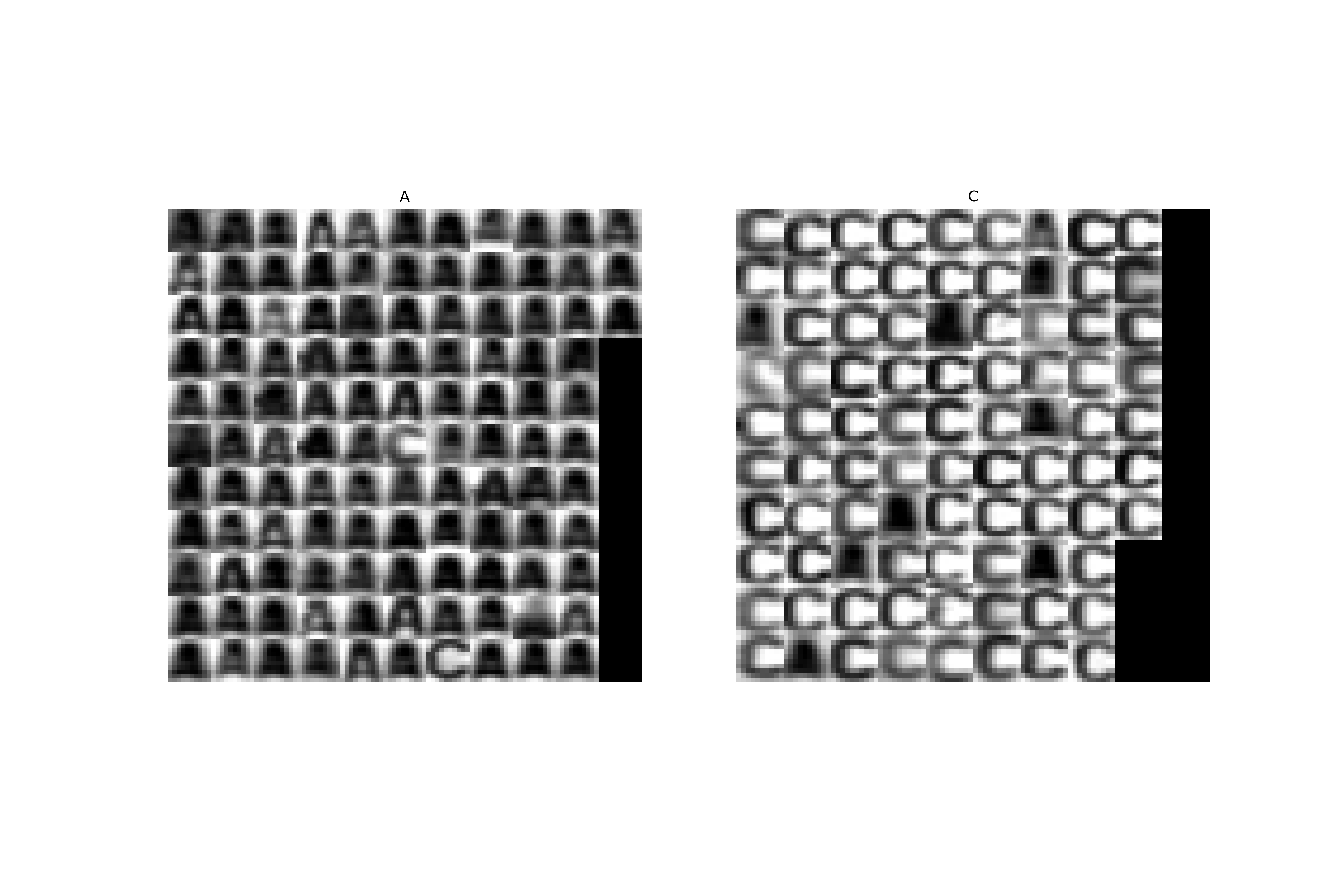


Part 3: Real world example - digit classification
Finally, we will apply all the above methods to a real world example similar to what you may encounter in typical pattern recognition problems. We will use the MNIST database of hand-written numerals and will train an SVM classifier with RBF kernel for two numerals 0 and 1. In this case the dimensionality of features is much higher as we are going to use the pixel intensities directly (i.e. we have 784-dimensional measurements). Thus we cannot really plot the separating hyperplane, but we can still learn the SVM, do the cross-validation and classify.
Note that we have already normalized the data for you such that each example has zero mean and unit variance. It is also important to mention here, that the pixel intensities are not the best features we could use. Better results could be obtained with more sophisticated features e.g. the image gradients, local binary patterns or histogram of oriented gradients or some combinations of multiple features together. We refer to Feature detection as a starting point for those who would like a deeper understanding of the feature acquisition topic.
We have also limited the training set just to a relatively small number of examples, while for testing we have much bigger set. This is, of course, not typical as we should use as many training examples as possible. The reason for this is purely educative to ease the computational expenses as we do not expect that you have access to some grid computing system. In machine learning it is quite usual that it takes several hours (even up to days) to learn a classifier. Also note that while in our case learning could be very time consuming, the evaluation on test data is very fast.
- Estimate the optimal values of the parameters $C$ and $\sigma$ (the width of the RBF kernel) on the MNIST training data
mnist_trn.npzby using the 5-fold 2D cross-validation for $C \in \{0.01,0.1,1, 10\}$ and $\sigma \in \{0.1, 1, 5, 10, 15, 20\}$.
- Train an SVM with a RBF kernel on the whole training data with optimal parameters $C^*$ and $\sigma^*$.
- Evaluate the trained SVM on the test data
mnist_tst.npz:
- Compute the classification error on the test data. You will need this value in the questions below.
- Show the classification of the digits with the optimal classifier and save it as
mnist_tst_classif.png
Hint: Use the functionshow_mnist_classificationto display the classification.

Assignment Questions
Fill the correct answers to your answers.txt file.
- Imagine that someone will give you a matrix $\mathbf{K}$ and you would like to use it in your Kernel SVM for the kernel matrix. What must hold in order to make it possible? Select all that apply.
- a) There are no other requests, as long as we have the $\mathbf{K}$, we can use it.
- b) $\mathbf{K}$ has to be negative-definite.
- c) $\mathbf{K}$ has to be symmetric.
- d) $\mathbf{K}$ has to be positive-semidefinite.
- e) This is not possible, since we would have no way how to obtain the feature mapping $\phi(\mathbf{x})$ from $\mathbf{K}$.