Table of Contents
HW 03 - Lidar Segmentation
Semantic Segmentation
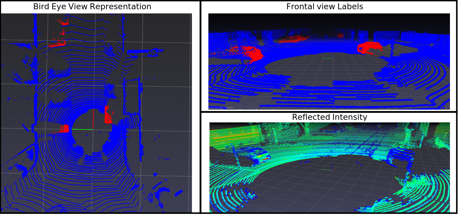
The goal of semantic segmentation is to classify every point in the input data to chosen classes in a supervised way (from labels). We will not use RGB images, but Lidar point clouds from autonomous driving scenarios, see illustration images, how it looks like. Good overview of the segmentation can be found: Here. It is not recommended, to read the details of the link. You can just consult it if you find easier explanation on RGB data than on lidar point clouds. Check our explanation Video
Lidar Data
Video. Your task is to train the model to segment the Vehicle class in the Bird Eye View representation. The Data are lidar point clouds from driving scenes and are in form of a 3D geometrical point cloud with lidar intensity (strength of returned laser) and per-point semantic labels. The autonomous driving scenario can be approximated into the 2D scene, since Vehicles and Pedestrians are moving on the plane. The Bird Eye view (BEV) is the 2d map representation of the data (See examples and codes). BEV can be formed as a tensor, where we input the features from the point cloud. The parameters of the BEV are in the following table:
| Parameters | range / value | Notes |
|---|---|---|
| x_range | (0,50) | Range of an area in x-axis |
| y_range | (-20,20) | Range of an area in y-axis |
| cell_size | (0.2,0.2) | Resolution of bin in tensor. Points are mapped into these bins |
| Channels | Your Implementation | Point Information in channels (similar to RGB in images) |
| shape of BEV | (250, 200) | The shape is automatically calculated from the 3 previous parameters |
The input data are therefore in a format of BEV with shape (250, 200, nbr_of_engineered_features). Your task is to map reasonable values into Bird Eye View channels (like Red color in RGB), so it will help the model to learn Vehicle class Segmentation. Suggested important features might be Intensity, Point occupancy (is there point or not), Density of Points, Maximum height in bin, Variance in bin.
The dataset consists of 1000 training point clouds, 100 testing and 148 validation point clouds. Each point cloud has a resolution of nx5, where n denotes number of points and each point has channels (x-coordinate, y-coordinate, z-coordinate, Intensity of reflection and Semantic label (1 for Vehicles, 0 for background). You can find it on servers on /local/temporary/vir/hw3 in .npy files.
Class mapping is following:
| Class ID | Class name | Color | Notes |
|---|---|---|---|
| 0 | No-Vision | Any place without reflected signal | |
| 1 | Background | 3D point with class other than Vehicles | |
| 2 | Vehicles | Only Cars. Data with Truck, Trams and other Vehicles types were filtered |
Data Augmentation
Useful trick to increase the generalization ability of the model is to augment the data. For example, you can rotate the point cloud along z-axis to prevent overfitting on the object in front of the ego car. Or you can scale or shift (translate) the point cloud so it create different view point on the data. Since we are using only front view, there is one easiest and quickest way, how to get more from the available 3D dataset. Think for yourself, how to leverage the data more efficiently.
Label Format
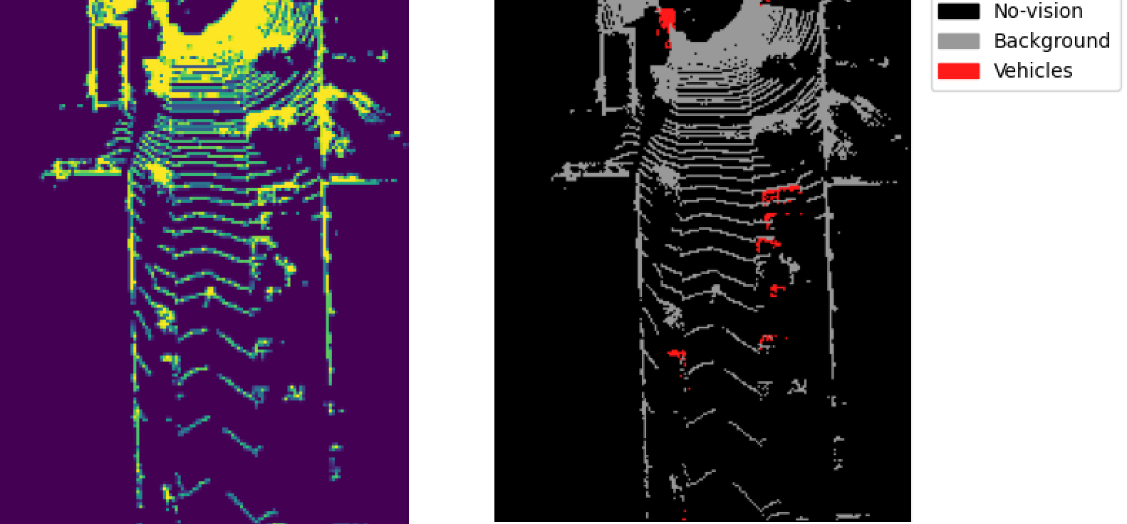
Here we show, how the labels looks like. It is a BEV tensor with shape (250,200), where values in bins corresponds to the classes. On the left, we see occupancy grid (point in the bin or not) and on the right, we see labels. The creation of the label is already included in the code.
Ilustration of the overfitting on single frame:
Recommended Architecture
Video. The Segmentation is a form of classification problem, where we intend to classify each bin of the target map representation. We can use the same mechanism as in Image classification, we just need to adjust the dimensions of the tensors to get the same output shape as in the input.
We recommend to implement the segmentation architecture with the style of U-Net. It is a typical “hour-glass” segmentation network for images. Here, we treat the Bird Eye View as a multi-channel image. It uses Skip Connections, which combine lower level features with high level ones in convolutions and improve the training process. The upsampling to the larger tensor dimension is handled by the Transposed Convolution, which “reverse” the standard convolution operation.
Class Imbalance
As you can imagine, the number of Vehicle class points is much smaller than the Background class. During the learning process, the model will tend to trade the smaller class for the one with majority of the points, because it contributes much more in the loss function. Therefore, we need to penalize the minority class false classification more in loss. There are two ways (orthogonal to each other) how to do it. First one is to introduce the class weights in Cross-entropy and the second is the extension called Focal Loss.
import torch
# The weight tensor here will keep the loss on first two categories as usual negative logarithm of probability.
# On the third one, it multiplies the loss by 100 to enforce model to increase the probability more on the particular class
# We recommend to keep in <0;1> for normalization consistency and proportional to number of occurence of that class
torch.nn.CrossEntropyLoss(weight=torch.tensor((1,1,100)))
The focal loss is a more “learnable” way how to tackle the same problem and it is already implemented in the codes. It introduces the hyper-parameter gamma for weighting the contribution of highly confident predictions or lower confidences. It is described on the following figure:
In order to use CrossEntropyLoss class for focal loss calculation, you can use the torch.nn.CrossEntropyLoss(reduction='none') which outputs the same 2d map of losses, not the mean of the tensor.
Sometimes, you can observe “nan” in the loss function. That is usually because of exploding gradients along deep network. You can use gradient clipping to keep the loss values at bay.
Metric
We will use Intersection-over-Union as a performance metric. It takes into account the False positives and False negatives as well. It is a combination of Precision and Recall in some form. It is denoted $IoU = \frac{TP}{TP + FP + FN} $. We present the evaluation script, which will be used in the brute
Submission
Video. You are given following codes as a templates. You will upload the weights.pth, load_model.py and load_data.py. The addition of your own Lidar_Dataset class in load_data.py with the function lidar_map will be used for creation of BEV for testing. The script load_data.py will contain only this class. Your Lidar_Dataset will be imported in BRUTE and will use your own BEV lidar_map function in evaluation. The only thing that needs to remain the are the labels, which are in the template script, so do not change them by any means!
Deadline
The deadline for this homework is 22.12. It is a lot of time not because it is time-consuming or hard. It is meant to give you space to catch up with other duties. If you decide to do it just before the deadline, consider the idea, that others might do similar thing and you will be left without the free GPU card on the server.


