Table of Contents
Maximum likelihood, Maximum a posteriori and Bayesian inference estimates of distribution parameters
At the very beginning of the recognition labs, we assumed the class probability densities $p_{X|k}(x|k)$ and the a priori probabilities $p_K(k)$ to be known and we used them to find the optimal Bayesian strategy. Later, we looked at problems where the a priori probability is not known or does not exist and we constructed the optimal minimax strategy. Today, we face the problem of unknown probability density function $p_{X|k}(x|k)$ and we will be interested in its estimation.
In this lab we will assume that we know the density function is from a class of functions characterized by several parameters, and we will be dealing with estimating their optimal value. In particular, we will consider two cases:
- the density is modeled by a Normal distribution – the unknown parameters will be the mean and variance of the distribution
- the density is modeled as a Categorical distribution – the unknown parameters will be the probabilities of individual classes/categories
To estimate the parameters we will use a training set - a set of examples drawn randomly from the particular distribution.
We will implement and evaluate three parameter estimation methods: Maximum likelihood (ML), Maximum a posteriori (MAP), and Bayesian inference.
The assignment has three parts. In the first one we will apply all the methods to the Normal distribution, in the second to the Categorical distribution and in the third part we will build a Bayes classifier using the estimated densities.
General information for Python development.
To fulfill this assignment, you need to submit these files (all packed in one .zip file) into the upload system:
mle_map_bayes.ipynb- a notebook for data initialization, calling of the implemented functions and plotting of their results (for your convenience, will not be checked).mle_map_bayes.py- file with the following methods implemented:ml_estim_normal- function which computes a ML estimate of Normal distribution parametersml_estim_categorical- function which computes a ML estimate of Categorical distribution parametersmap_estim_normal- function which computes a MAP estimate of Normal distribution parametersmap_estim_categorical- function which computes a MAP estimate of Categorical distribution parametersbayes_posterior_params_normal- function which computed the a posteriori distribution parameters using Bayesian inference for Normal distributionbayes_posterior_params_categorical- function which computed the a posteriori distribution parameters using Bayesian inference for Categorical distributionbayes_estim_pdf_normal- function which computes a Bayesian estimate for Normal distribution as a NIG probability density functionbayes_estim_categorical- function which computes a Bayesian estimate of Categorical distribution parametersmle_Bayes_classif- function which classifies using ML estimate of normal distributionsmap_Bayes_classif- function which classifies using MAP estimate of normal distributionsbayes_Bayes_classif- function which classifies using Bayes estimate of normal distributions
mle_normal_derivation.jpg,map_normal_derivation.jpg,mle_categorical_derivation.jpgandmap_categorical_derivation.jpg- images of handwritten derivationsmle_normal.png,mle_normal_varying_dataset_size.png,map_prior_normal.png,mle_map_prior_comparison_normal.png,mle_map_normal_dataset_sizes.png,bayes_posterior_normal.png,mle_map_bayes_normal.png,noise.png,categorical_data.png,mle_categorical.png,map_categorical.png,bayes_posterior_categorical.png,bayes_categorical.pngandmle_map_bayes_Bayes_classifier.png- images specified in the assignment
Use template of the assignment. When preparing a zip file for the upload system, do not include any directories, the files have to be in the zip file root.
bayes.py in BRUTE, please copy all the necessary functions directly into mle_map_bayes.py. Sorry for the inconvenience.
Part 1: Normal distribution
At first, we will use synthetic data to examine the basic properties of different estimates. Start by generating some i.i.d. data $X=\{x_1, \ldots, x_N\}$ from a unimodal Normal distribution with $\mu=0$ and $\sigma^2=1$, i.e. $x_i \sim \mathcal{N}(\mu, \sigma^2)$. For most demonstrations $N=50$ data points will be enough. But feel free to experiment with larger datasets.
Maximum Likelihood Estimation
As you know from the lecture, our goal in MLE is to find a solution to this problem: $$\mu_*, \sigma_* = argmax_{\mu, \sigma} p(X| \mu, \sigma) = argmax_{\mu, \sigma} \prod_{i=1}^N p(x_i| \mu, \sigma)\;,$$ where the likelihood $p(x_i|\mu, \sigma)$ is the Normal distribution $\mathcal{N}(x_i|\mu, \sigma)$.
- Start by deriving the maximum likelihood estimates of the Normal distribution parameters $\mu$ and $\sigma^2$. Use the formulas to complete the function
ml_estim_normal.
- Submit a photo of handwritten derivation notes in
mle_normal_derivation.jpg(this is a good chance to see, how log-likelihood could be useful ;) )mu_mle, var_mle = ml_estim_normal(np.array([1, 4, 6, 3, 4, 7])) # -> 4.166666666666667, 3.805555555555556
- Use the function
plot_likelihoodto plot the likelihood for a range of $\mu$ and $\sigma^2$ values. Mark the true and estimated values. Next, plot the true and estimated distributions in one graph.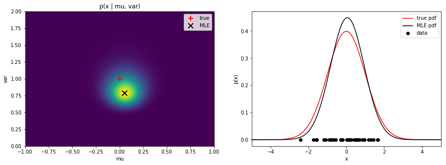 Save the figure as
 mle_normal.png.
Hint: Useplt.subplots.
- Try to generate the data repeatedly while re-drawing these plots. Observe the variations in the estimate. After seeing this, how much would you trust an ML estimate? Did you know that MLE is probably the most frequently used parameter estimation technique?
- A common way to avoid imprecise ML estimates is to increase the number of data points. Try to plot the true and estimated distributions with increasing number of samples.
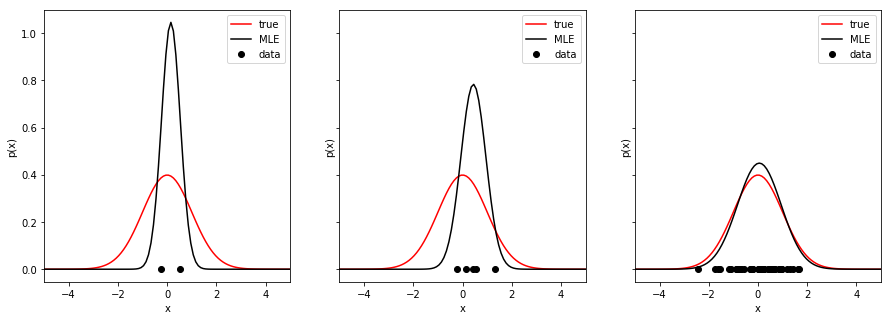 Save the figure as
 mle_normal_varying_dataset_size.png.
MAP Estimation
As you know from the lecture, in the MAP estimation the parameters are found by maximizing the a posteriori probability:
$$\theta_* = {\rm argmax}_{\theta} p(\theta | X) = {\rm argmax}_{\theta} p(X| \theta) p(\theta)$$
The advantage is that we can specify our prior knowledge about the true values of the parameters in the form of the prior $p(\theta)$ and thus avoid wrong uninformed estimates in case too few samples are available.
It was argued in the lecture that in order to obtain a close-form expression for a posterior probability, one should use a conjugate prior. In the lecture when we were estimating $\theta = \mu$ only and $\sigma^2$ was assumed to be known, a Normal distribution prior was used, which simplified the derivation significantly. In our current case, we assume $\theta = (\mu, \sigma^2)$, i.e. that both $\mu$ and $\sigma^2$ are unknown. Fortunately, even in this case there exists a conjugate prior. Out of several possible choices we will use the normal inverse gamma distribution:
$$p(\mu, \sigma^2) = \mbox{NIG}(\mu, \sigma^2 | \mu_0, \nu, \alpha, \beta) = \frac{\sqrt{\nu}}{\sigma \sqrt{2\pi}} \frac{\beta^\alpha}{\Gamma(\alpha)} \left(\frac{1}{\sigma^2}\right)^{\alpha+1} \exp\left[-\frac{2\beta + \nu(\mu_0 - \mu)^2}{2\sigma^2}\right]$$
where $\mu_0, \nu, \alpha$ and $\beta$ are the distribution parameters and $\Gamma(\cdot)$ is the Gamma function which is implemented in scipy.special.gamma.
A consequences of this choice, which we will explore in more detail in the next section on Bayesian inference, is that the a posteriori probability is again NIG, just with different parameters.
It is interesting to get the intuition behind the prior parameters. One can think of them as if before any data have been seen, the mean $\mu$ was estimated from $\nu$ observations with sample mean $\mu _{0}$ and the variance $\sigma^2$ was estimated from $2\alpha$ observations with sample mean $\mu _{0}$ and sum of squared deviations $2\beta$.
Alternatively, we may be interested in providing a prior values for $\mu$ and $\sigma^2$ (denoted $\mu_{my}, \sigma_{my}^2$) and then control the shape of the distribution around this peak. In this case, we set $\mu_0 = \mu_{my}$ and the parameters $\alpha$ and $\beta$ are linked by $\beta = \sigma_{my}^2 * (\alpha + 1.5)$, while $\nu$ stays a free parameter (this comes from the equations of the mode of the NIG distribution). So, using this parametrization we would specify e.g. $\mu_{my}, \sigma_{my}^2, \alpha$ and $nu$ instead of the original four parameters.
The prior pdf is implemented in norm_inv_gamma_pdf. Go and check that the implementation fits the formulas listed above.
Tasks:
- Plot the distribution using the provided
plot_priorfunction together with its mode. Save the figure asmap_prior_normal.png.
- Experiment with different settings of $\mu_0, \nu, \alpha, \beta$ to get the feeling for how each of the parameters influences the prior. You will need this understanding later when we will be building a classifier using the MAP estimate.
- Show that the MAP estimate of the parameters $\mu$ and $\sigma^2$ with the normal inverse gamma prior is $$\mu_* = \frac{\nu\mu_0 + \sum_{i=1}^N x_i}{N + \nu}$$ $$\sigma_*^2 = \frac{2\beta + \nu(\mu_0 - \mu_*)^2 + \sum_{i=1}^N (x_i - \mu_*)^2}{N + 3 + 2\alpha}$$ Submit a photo of handwritten derivation notes in
map_normal_derivation.jpg.
- Implement the
map_estim_normalfunction which returns the MAP estimate of the parameters given the data and the prior probability parameters.mu_map, var_map = map_estim_normal(np.array([2, 7, 3, 5, 1, 0]), mu0=0, nu=5, alpha=1, beta=2.5) # -> (1.6363636363636365, 5.77685950413223)
- Plot the likelihood, prior and the MAP objective $p(X| \theta) p(\theta)$ next to each other, together with the MLE and MAP estimates and the prior maximum. Save the figure as
mle_map_prior_comparison_normal.png.
Notice: The MAP objective is not a distribution as it does not integrate to one because we omitted the evidence $p(X)$!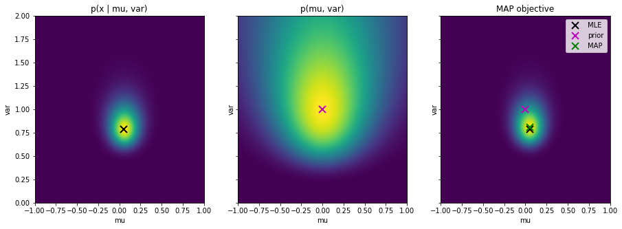
- Examine the behavior of the MAP estimate compared with the ML estimate and the prior. Experiment with
- repeatedly sampling the dataset and observing the variations in the estimate
- changing the prior parameters to see their effect on the estimate
- To explore the effect of the prior, plot the MLE and MAP estimates for different dataset sizes (e.g. 1, 5, 50). Plot the MAP objective with the estimates and prior indicated. Plot also the estimated distributions for each dataset size. You should see how the prior becomes more dominant the less data samples are available. Notice that for a single data sample $X = \{x_1\}$ we do not plot the MLE solution. It would actually be $\sigma^2=0$ and $\mu=x_1$, so we would get an infinitely thin and infinitely tall normal distribution centered on the data point. This is of course not a realistic estimate. Save the figure as
mle_map_normal_dataset_sizes.png.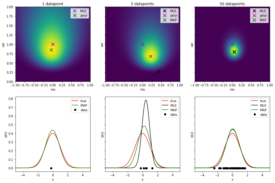
Bayesian Inference
In the Bayesian inference, we are interested in computing a posteriori distribution $p(\mu, \sigma^2 | X)$ over possible parameter values. We use the Bayes' rule:
\begin{align*} p(\mu, \sigma^2 | X, \mu_0, \nu, \alpha, \beta) &= \frac{\prod_{i=1}^N p(x_i|\mu, \sigma^2) p(\mu, \sigma^2)}{p(X)} \\ &=\frac{\prod_{i=1}^N \mathcal{N}(x_i|\mu, \sigma^2) \mbox{NIG}(\mu, \sigma^2 | \mu_0, \nu, \alpha, \beta)}{p(X)} \\ &= \frac{\kappa \; \mbox{NIG}(\mu, \sigma^2 | \tilde{\mu}_0, \tilde{\nu}, \tilde{\alpha}, \tilde{\beta})}{p(X)} \end{align*}
where the conjugate relationship between the likelihood and prior has been used and $\kappa$ is the associated normalization constant. The parameters of the new normal inverse gamma distribution can be shown to be
\begin{align*} \tilde{\alpha} = \alpha + N/2 \qquad \tilde{\nu} = \nu + N \qquad \tilde{\mu}_0 = \frac{\nu \mu_0 + \sum_i x_i}{\nu + N} \\ \tilde{\beta} = \beta + \frac{\sum_i x_i^2}{2} + \frac{\nu \mu_0^2}{2} - \frac{(\nu \mu_0 + \sum_i x_i)^2}{2(\nu + N)} \end{align*}
Notice further, that the a posteriori is a distribution, i.e. it integrates to one, so also the right hand side of the equation must be a distribution and thus the constant $\kappa$ and the denominator must exactly cancel out. So, thanks to the conjugacy of the prior, we again arrive at a close-form solution to the a posteriori distribution:
$$ p(\mu, \sigma^2 | X, \mu_0, \nu, \alpha, \beta) = \mbox{NIG}(\mu, \sigma^2 | \tilde{\mu}_0, \tilde{\nu}, \tilde{\alpha}, \tilde{\beta}) $$
Task:
- Implement the above formulas into
bayes_posterior_params_normaland use the functionplot_posterior_normalto plot the a posteriori probability over $\mu$ and $\sigma^2$ values. Mark the MLE, MAP and maximum prior solutions.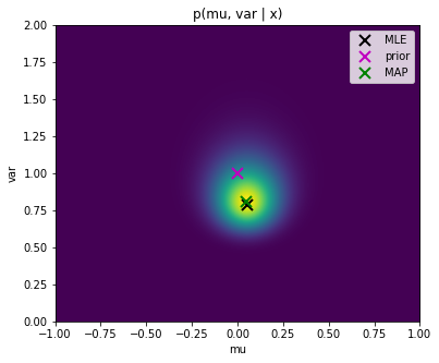 Save the figure as
 bayes_posterior_normal.png.
Notice, that the graph looks exactly the same as for the MAP objective we created above. This is due to the normalisation of the plots in matplotlib. However, as notices above, the MAP objective is not a probability distribution as it does not integrate to one. On the other hand, the a posteriori $p(\mu, \sigma^2 | X, \mu_0, \nu, \alpha, \beta)$ is a correct distribution which integrates to one.
One interpretation of this graph is that, truly, the most likely solution is the MAP estimate, but there are also other possible solutions which only have smaller probability. What we want to do is to take them into account when making the prediction of the estimated distribution.
Predictive density
In the Bayesian inference we do not take only the most probable estimate of $\mu$ and $\sigma^2$ and use it for evaluation of $p(x|\mu, \sigma^2)$, but we compute a weighted average of the predictions at a test point $x^*$ for each possible parameter settings, where the weighting is given by the above posterior distribution.
\begin{align*} p(x^* | X, \mu_0, \nu, \alpha, \beta) &= \int \int p(x^* | \mu, \sigma^2) p(\mu, \sigma^2 | X, \mu_0, \nu, \alpha, \beta) d\mu d\sigma \\ &= \int \int \mathcal{N}(x^*|\mu, \sigma^2) \mbox{NIG}(\mu, \sigma^2 | \tilde{\mu}_0, \tilde{\nu}, \tilde{\alpha}, \tilde{\beta}) d\mu d\sigma \\ &= \int \int \kappa(x^*, \tilde{\mu}_0, \tilde{\nu}, \tilde{\alpha}, \tilde{\beta}) \mbox{NIG}(\mu, \sigma^2 | \breve{\mu}_0, \breve{\nu}, \breve{\alpha}, \breve{\beta}) d\mu d\sigma \end{align*}
where we used the conjugate relation for the second time (adopted from Prince book). We will call this distribution predictive density. Taking the constant out of the integrals we get
\begin{align*} p(x^* | X, \mu_0, \nu, \alpha, \beta) &= \kappa(x^*, \tilde{\mu}_0, \tilde{\nu}, \tilde{\alpha}, \tilde{\beta}) \int \int \mbox{NIG}(\mu, \sigma^2 | \breve{\mu}_0, \breve{\nu}, \breve{\alpha}, \breve{\beta}) d\mu d\sigma \\ &= \kappa(x^*, \tilde{\mu}_0, \tilde{\nu}, \tilde{\alpha}, \tilde{\beta}) \end{align*}
as the integral over the distribution is one and the constant $\kappa$ is given by
$$ \kappa(x^*, \tilde{\mu}_0, \tilde{\nu}, \tilde{\alpha}, \tilde{\beta}) = \frac{1}{\sqrt{2\pi}} \frac{\sqrt{\tilde{\nu}}\tilde{\beta}^{\tilde{\alpha}}}{\sqrt{\breve{\nu}}\breve{\beta}^{\breve{\alpha}}} \frac{\Gamma(\breve{\alpha})}{\Gamma(\tilde{\alpha})} $$
and
\begin{align*} \breve{\alpha} = \tilde{\alpha} + 1/2 \qquad \breve{\nu} = \tilde{\nu} + 1 \\ \breve{\beta} = \frac{{x^*}^2}{2} + \tilde{\beta} + \frac{\tilde{\nu}\tilde{\mu}_0^2}{2} - \frac{(\tilde{\nu}\tilde{\mu}_0 + x^*)^2}{2(\tilde{\nu} + 1)} \end{align*}
Tasks:
- Implement the function
bayes_estim_pdf_normalusing the above equations.
- Plot the estimated pdf for MLE, MAP and Bayes inference into one graph. Beware that the Bayes estimate is not a Normal distribution anymore! Make plots for different dataset sizes. Save the figure as
mle_map_bayes_normal.png.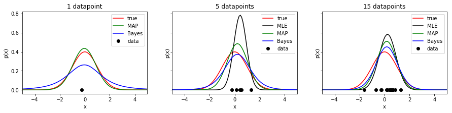
- However, imagine that for some reason, part of your data is corrupted by errors/noise. Add a single out-of-distribution sample further from the distribution mean. Plot the estimated distributions using this corrupted dataset. Save the figure as
noise.png.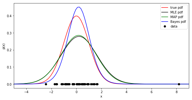
Take-away summary
- MLE is easy to compute, but it requires large datasets to produce a reliable estimate. With small datasets, it produces often wrong but over-confident (high values of pdf) predictions.
- MLE is sensitive to outliers.
- MAP allows to include a prior on the estimated parameters and can thus produce reasonable predictions even on smaller datasets.
- MAP is also sensitive to outliers as we rely on a single estimate and neglecting the rest of the distribution over the parameters.
- In the limit, when increasing the data size, MLE converges to MAP solution.
- When given a uniform prior, MAP becomes MLE (shown in the lecture slides). Bayesian inference can work even with a uniform prior, however, having a good prior improves the estimate.
- Bayesian estimates tend to be rather conservative (notice the heavier tails of the distribution) giving some probability to even data values not observed yet.
- Ideally, we would like to use the Bayesian inference, but its need for a conjugate prior is limiting and thus we often resort to a less robust method. This then pushes up our needs for large datasets.
- Alternatively, we may resort to a numerical solution of the Bayesian inference when we do not have a conjugate prior.
- Another question is, what is a good prior for a particular problem… We will see later how a wrong prior influences a Bayesian classifier which uses a MAP estimate.
Part 2: Categorical distribution
Next, lets look at estimating parameters of a categorical distribution. Suppose that our dataset $X=\{x_1, \ldots, x_N\}$ consists of points $x_i \in \{1, 2, \ldots, K\}$, like if we were throwing a biased dice or estimating preferences of $K$ presidential candidates. The categorical distribution is defined as
$$ p(x = k| p_1, \ldots, p_K) = p_k \qquad \mbox{where} \quad \sum_{k=1}^K p_k = 1$$
For the ML and MAP we estimate the parameters $\{p_k\}_{k=1}^K$, for the Bayesian approach we compute a probability distribution over the parameters.
Tasks:
- Start by generating data (e.g. 50 points) from a known categorical distribution with $K=6$ (e.g. a biased dice). Make one of the class probabilities intentionally very small (e.g. 0.01) to be able to observe the effect of zero training samples for one bin.
- Plot side-by-side the distribution itself and the histogram of the measured data (btw, categorical distribution is sometimes referred to as a 'normalized histogram'). Save the figure as
categorical_data.png.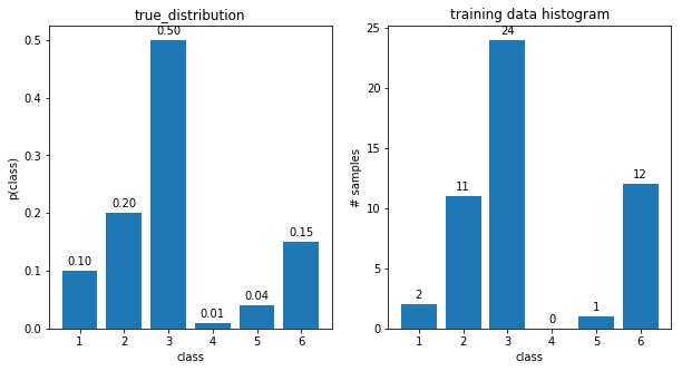
MLE
Tasks:
- Show that the maximum likelihood estimate of the parameters $p_k$ is $$ \hat{p}_k = \frac{N_k}{\sum_{m=1}^K N_m} $$ where $N_k$ is the number of measurements of the class $k$. Submit a photo of handwritten notes as
mle_categorical_derivation.jpg
Hint: Use the Lagrange multiplier method (or here)for the constraint $\sum_k p_k = 1$ and combine the derivatives over $p_k$ and the Lagrange multiplier $\lambda$. It is also easier to optimize the log of likelihood.
- Complete the function
ml_estim_categoricaland use it to estimate the distribution parameters.
- Plot the estimated distribution. Save the figure as
mle_categorical.png.
MAP
As a prior needed for MAP estimation we choose the Dirichlet distribution as it is conjugate to the categorical likelihood
$$ \mbox{Dir}(p_1, \ldots, p_K; \alpha_1, \ldots, \alpha_K) = \frac{1}{B(\alpha)} \prod_{k=1}^K p_k^{\alpha_k - 1} $$
where $B(\alpha)$ is a normalization constant and $\alpha = (\alpha_1, \ldots, \alpha_K)$. It is implemented in numpy.random.dirichlet.
Tasks:
- As with the previous prior, we start by examining its behavior for various parameter settings. Sample five random distributions from this prior and plot them side-by-side. Experiment with the parameters $\alpha$:
- start with $\alpha_k = 1$ for all $k$
- keep all the values the same, but increase their value
- try to set one of $\alpha_k$'s significantly higher
- try to set all $\alpha_k$ below 1 (this will not work with MAP estimate - you may get negative probability estimate)
Thus a fair dice would correspond to $\alpha_k \rightarrow \infty$ and when all $\alpha_k$'s are the same and greater than one, the distribution produces a fair dice on average. When the prior is uniform, i.e. when $\alpha_k = 1$ for all $k$, the MAP derivation reduces to the ML estimate.
Some more intuition for Dirichlet distribution as a conjugate prior is given in this blog post.
- Show that the MAP estimate of the parameters $p_k$ is $$ \hat{p}_k = \frac{N_k + \alpha_k - 1}{\sum_{m=1}^K (N_m + \alpha_m - 1)} $$ where $N_k$ is the number of measurement of the class $k$.
Hint: The derivation is similar to the MLE estimate.
- Submit a photo of handwritten derivation notes as
map_categorical_derivation.jpg.
- Complete the function
map_estim_categoricaland use it to estimate the distribution parameters.
- Plot the estimated distribution. Save the figure as
map_categorical.png.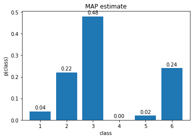
Bayesian inference
In the Bayesian approach we calculate a posteriori probability over the parameters (derivations adopted from Prince book)
\begin{align*} p(p_1, \ldots, p_6| X) &= \frac{\prod_{i=1}^N p(x_i|p_1, \ldots, p_6) p(p_1, \ldots, p_6)}{p(X)} \\ &= \frac{\prod_{i=1}^N \mbox{Cat}(x_i|p_1, \ldots, p_6) \mbox{Dir}(p_1, \ldots, p_6; \alpha_1, \ldots, \alpha_6)}{p(X)} \\ &= \frac{\kappa(\alpha_{1},\ldots, \alpha_{6}, X) \mbox{Dir}(p_1, \ldots, p_6; \tilde{\alpha}_1, \ldots, \tilde{\alpha}_6)}{p(X)} \\ &= \mbox{Dir}(p_1, \ldots, p_6; \tilde{\alpha}_1, \ldots, \tilde{\alpha}_6) \end{align*}
where $\tilde{\alpha}_k = N_k + \alpha_k$ and where we have once again exploited the conjugate relationship between the likelihood and prior. And as before, the normalization constant $\kappa$ cancels out with the denominator in order to obtain a valid probability distribution.
The predictive density used in ML and MAP was simply the categorical distribution with the estimated parameters $\hat{p}_k$. In the Bayesian case, we compute a weighted average of the predictions for each possible parameter set, where the weighting is given by the posterior distribution.
\begin{align*} p(x^*|X) &= \int p(x^*|p_1, \ldots, p_6) p(p_1, \ldots, p_6| X) dp_{1\ldots 6} \\ &= \int \mbox{Cat}(x^*|p_{1\ldots 6}) \mbox{Dir}(p_{1\ldots 6}; \tilde{\alpha}_{1\ldots 6}) dp_{1\ldots 6} \\ &= \int \kappa(x^*, \tilde{\alpha}_{1\ldots 6}) \mbox{Dir}(p_{1\ldots 6}; \breve{\alpha}_{1\ldots 6}) dp_{1\ldots 6} \\ &= \kappa(x^*, \tilde{\alpha}_{1\ldots 6}) \end{align*}
and it can be shown that
$$ p(x^*=k|X) = \kappa(x^*, \tilde{\alpha}_{1\ldots 6}) = \frac{N_k + \alpha_k}{\sum_{j=1}^6 (N_j + \alpha_j)} $$
Tasks:
- Implement the
bayes_posterior_params_categoricalfunction.
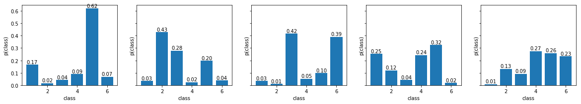
- Sample five samples from this posterior and display them side-by-side. Compared with the samples from the prior, they should resemble better the data distribution. Save the figure as
bayes_posterior_categorical.png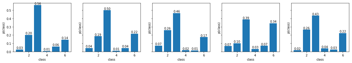
- Implement the function
bayes_estim_categoricalwhich returns the Bayesian estimate.
- Plot the estimated distribution. Save the figure as
bayes_categorical.png.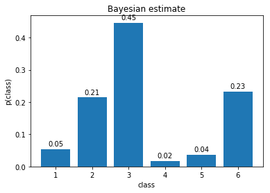
- Experiment with different priors.
Take-away summary
- Notice that even with flat uninformative prior (i.e. when $\alpha_1 = \ldots = \alpha_6 = 1$), Bayesian approach tends to give non-zero probability to bins for which no data has been observed yet.
- In contrast, in MAP estimate the flat prior resulted in the same result as in ML estimate.
Part 3: Building a classifier
In this part we will use the MLE, MAP and Bayesian estimates for the Normal distribution to build a Bayes classifier as in the previous assignment. Feel free to use your code from the previous lab to finish this task. However, upload every function needed so that we can evaluate it automatically.
The task is again to distinguish the images of letters 'A' from images of 'C' using the compute_measurement_lr_cont measurement.
Spend some time specifying a meaningful prior for MAP and Bayesian estimates for both classes. The old values (0, 1) will no longer work here as the mean and variance of the data is different (in thousands)! It is recommended to plot the prior for a visual feedback for the parameters.
Tasks:
- Implement the functions
mle_Bayes_classif,map_Bayes_classifandbayes_Bayes_classif. Assume 0/1 loss function. The first two will use the strategy from the Bayes classification labs, whereas for the bayesian estimate the pdf is no longer a Normal distribution, so we have to use the inequality $p(A)p(x|A) > p(C)p(x|C)$ for deciding for the class. Compute the a priori probabilities as relative frequencies in the training dataset.
- Compute the classification error on the test set for all three methods.
- Visualize the data through normalized histograms, plot the estimated probability densities and the estimated strategies all in one plot. Save the figure as
mle_map_bayes_Bayes_classifier.png.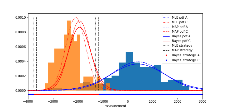
- Experiment with setting the MAP prior probability parameters in various ways to get the feeling for how they influence the final classification.
- Experiment with different training dataset sizes (20, 200, 2000 samples). Observe the influence of the prior parameters on the classification given different dataset sizes.
References
Simon J.D. Prince. Computer Vision: Models, Learning, and Inference. Cambridge University Press, 2012