Table of Contents
The Minimax Task
The Bayesian formulation has some limits discussed at the lecture and for certain situation one may need to formulate the problem e.g. as a Neyman-Pearson task, Wald task or minimax task. Out of this spectrum of problem formulations we will examine the minimax task.
To continue with our simple OCR developed in the previous labs, lets consider a situation when we are trying to recognise licence plates. For simplicity we again stick to the simple two-letter alphabet and 10×10 already segmented letters. The situation in the Bayes task then corresponds to a problem of designing a recognition system for a particular crossroad where the a priori probability of the two letters is known or could be measured.
In today's assignment we aim at designing a recognition system which could be deployed anywhere in the Czech republic and we need to take into account that licence plates in different cities use different combination of the letters, so the a priori probabilities differ as well. Further, lets assume it is not practical to find the optimal Bayesian strategy for each used camera.
As you might have already guessed, the situation is ideal for the minimax strategy. Here, the a priori probability exists, but is not known. We will first study the task rather theoretically to demonstrate some principles from the lecture and then we apply the gained knowledge to the real task of recognising the letters on the licence plates.
General information for Python development.
To fulfil this assignment, you need to submit these files (all packed in one .zip file) into the upload system:
answers.txt- answers to the Assignment Questionsminimax.ipynb- a notebook for data initialisation, calling of the implemented functions and plotting of their results (for your convenience, will not be checked).minimax.py- file with the following methods implemented:risk_fix_q_discrete,risk_fix_q_cont- functions for computing risk for a fixed strategy but changing a priori probabilityworst_risk_discrete,worst_risk_cont- worst case risk for a Bayesian strategy trained with a particular a priori probability but evaluated on all a priori probabilitiesminmax_strategy_discrete,minmax_strategy_cont- functions which find the optimal minmax strategy- all functions from the previous assignment (bayes) - Unfortunately, including bayes.py and import from it is not supported. You have to copy your functions from bayes.py to minimax.py.
plots_discrete.png,plots_cont.png,minmax_classif_cont.pngandminmax_classif_discrete.png- images specified in the tasks
Use template of the assignment. When preparing a zip file for the upload system, do not include any directories, the files have to be in the zip file root.
bayes.py in BRUTE, please copy all the necessary functions directly into minimax.py. Sorry for the inconvenience.
The Tasks
As in the last labs, use the discrete and continuous measurements $x$ computed by compute_measurement_lr_discrete and compute_measurement_lr_cont.
For the experiments, choose two letters corresponding to your initials and use the distribution parameters given in the following variables (assuming your name is Chuck Norris) for the discrete measurements tasks:
| variable | description |
|---|---|
discreteC['Prob'] | $p_{X|k}(x|C)$ given as a (21, ) numpy array (the size corresponds to the range of the values of $x$) |
discreteN['Prob'] | $p_{X|k}(x|N)$ given as a (21, ) numpy array (the size corresponds to the range of the values of $x$) |
and the following ones for the cases with continuous measurements:
| variable | description |
|---|---|
contC['Mean'] | mean value of the normal distribution $p_{X|k}(x|C)$ |
contC['Sigma'] | standard deviation of the normal distribution $p_{X|k}(x|C)$ |
contN['Mean'] | mean value of the normal distribution $p_{X|k}(x|N)$ |
contN['Sigma'] | standard deviation of the normal distribution $p_{X|k}(x|N)$ |
(still assuming you are Chuck Norris)
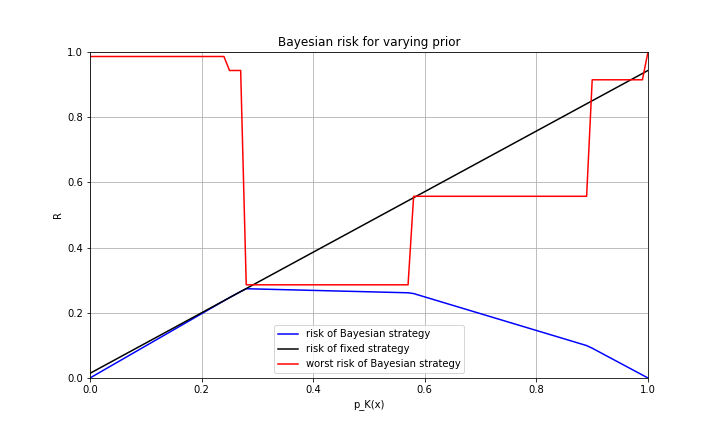
- Use the discrete distributions and for $p_K(C) \in \{0, 0.01, \ldots, 0.99, 1\}$ compute and plot into one figure the following:
- Risk of the Bayesian strategy optimal for each $p_K(C)$.
Hint 1: Use your code from the last labs.
Hint 2: In the minimax problem formulation, each error is penalised equally independent of the class (this corresponds to the 0-1 loss function).
- Find the optimal strategy for $p_K(C) = 0.25$. Then for this, now fixed strategy, alter the a priori probability and compute its Bayesian risk. For this complete the template function
risk_fix_q_discrete.
Hint 1: This is what happens, when we have assumed wrong a priori probabilities different from the real one.
Hint 2: Equation (3) from [1] explains the shape of the observed curve.
- For each iterated $p_K(C)$ derive the optimal Bayesian strategy and compute its worst-case risk in case the true a priori probability is different. For this complete the template function
worst_risk_discrete.
Hint: You can again use the equation (3) from [1] and the fact that the a priori probability is bounded to the <0,1> interval.
- Save the figure to
plots_discrete.png.
Assuming your name is Mirek Dušín. Chuck Norris initials refused to be used in this graph.
- Repeat the steps 1 and 2 for the continuous distributions and save the figure to
plots_cont.png. The implemented functions are the same but with_continstead of_discretesuffix.
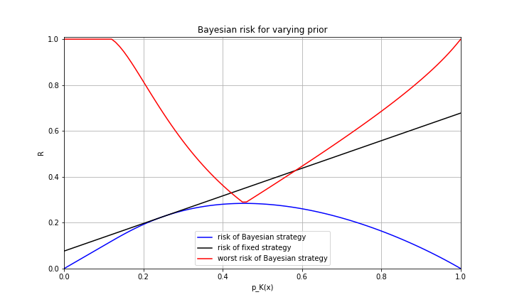
Assuming your name is Mirek Dušín. Chuck Norris initials refused to be used in this graph.
- Complete the template functions
minmax_strategy_discreteandminmax_strategy_cont, so that they find the minmax strategy and its risk for discrete and continuous measurements respectively. Hint: The minimax strategy is the Bayesian strategy with minimal maximal Bayesian risk over all $p_K(C)$.
Hint: usescipy.optimize.fminbound


D1 = discrete['C']
D2 = discrete['N']
q, risk = minmax_strategy_discrete(D1, D2)

# q -> array([0, 0, 0, 0, 0, 0, 0, 0, 0, 1, 1, 1, 1, 1, 0, 0, 0, 0, 0, 0, 0])
# risk -> 0.02857142873108387

D1 = cont['C']
D2 = cont['N']
q, risk = minmax_strategy_cont(D1, D2)

# q['t1'] -> -775.9750275387074
# q['t2'] -> 10080.038857544445
# q['decision'] -> array([0, 1, 0], dtype=int32)
# risk -> 0.013218704611063004
- Plot bayesian risk for all values of $p_K(C)$ for the minimax strategy in both discrete and continuos cases.
- Generate a test set for your initials using
create_test_set. - Compute the error of the strategy on the generated test images, show the final classification in one figure and save it as
minmax_classif_cont.pngandminmax_classif_discrete.png.
Hint: use theclassification_error_discreteandclassification_error_2normalfunctions from the bayes assignment.
error_discrete = classification_error_discrete( images_test_set, labels_test_set, q_minimax_discrete)
# error_discrete -> 0.0667

error_cont = classification_error_2normal( images_test_set, labels_test_set, q_minimax_cont)
# error_cont -> 0


Assignment Questions
Fill the correct answers to your answers.txt file.
- What is the maximal risk of the optimal Bayesian strategy trained for $P_K(A)=0.3$ and $P_K(B)=0.7$ using continuous measurement when the a priori probabilities are allowed to change? Round it to two decimal points.
- The relation between the worst case risk and the best case risk for the minimax strategy in the continuous case is
- a) The worst case risk is always greater than the best case risk
- b) The worst case risk could be smaller than the best case risk
- c) The worst case risk is strictly equal to the best case risk
- In the above we assumed the a priori probability exists but is not known. What would change if it didn't exist?
- a) We can't compute the risk and have to use the likelihood ratio directly
- b) We would need to use different loss function W
- c) We would proceed the same way as we did above
Bonus Task
This task is not compulsory.
Go through the chapter on non-Bayesian tasks in SH10 book [2], especially the parts discussing solution of the minimax task by linear programming (pages 25, 31, 35-38, 40-41, 46-47). Solve the above classification task using linear programming as described on page 47.
Hints:
- Work with the discrete measurements $x$.
- Represent the sought strategy (classification function) as a table α, with α(i,k) corresponding to the probability of classification of bin 'i' to class 'k' such that α(i,k) >= 0 and sum_k α(i,k) = 1.
- Reformulate the task in a matrix form according to equation 2.53 in SH10, page 47
- Solve the task numerically using
scipy.optimize.linprog. - Compare the obtained results with the results of the classification above.
References
- [1] Minimax Task (short support text for labs)
- [2] Michail I. Schlesinger, Vaclav Hlavac. Ten Lectures on Statistical and Structural Pattern Recognition. Kluwer Academic Publishers, 2002.