Homework 06 - Panorama
Input Images
Consider the images were captured with the following EXIF info (focal length is in milimeters):
| Tag | Name | Value |
|---|---|---|
| 0xa002 | ExifImageWidth | 2400 |
| 0xa003 | ExifImageHeight | 1800 |
| 0xa20e | FocalPlaneXResolution | 2160000/225 |
| 0xa20f | FocalPlaneYResolution | 1611200/168 |
| 0xa210 | FocalPlaneResolutionUnit | inch |
| 0x920a | FocalLength | 7400/1000 |
The images were then resized.
| 07 | 06 | 05 | 04 - reference | 03 | 02 | 01 |
 |  |  |  |  |  |  |
Steps
- Manually create 10 image matches (point correspondences) between every pair of adjacent images. Store in the cell matrix u such that
u{i,j}are points in the i-th image andu{j,i}are corresponding points in the j-th image. Save in06_data.mat - Find homographies
H_ijfor every pair of adjacent images by the same method (optimizing 4 over 10) as in HW-05; use youru2h_optimfunction for each homography. - Draw 6 histograms of transfer errors of all correspondences into a single image. Use different colour for every histogram, export as
06_histograms.pdf. - Compute homographies
H_i4for every i ∈ <1,7> that maps the images above into the reference image 04 (thusH_44is identity). Then construct inverse homographiesH_4i. - Store all homographies into the cell matrix
H, whereH{i,j}is the homography from i to j. Save in06_data.mat. - Plot the image borders of the images 02 to 06 transformed to the image plane of the image 04. Export as
06_borders.pdf. - Construct a projective panoramic image from the images 03, 04, and 05, in the image plane of the image 04. Save as
06_panorama.png. - Construct calibration matrix
Kusing the actual image size and the original EXIF. All the images share the same calibration. Store it in06_data.mat - Establish a transformation between each image plane and the coordinate system of the cylinder, described below.
- Plot the image borders of all the images mapped onto the cylinder (
06_borders_c.pdf). - Construct a panoramic image from all the images mapped onto the cylinder (
06_panorama_c.png). - Optionally, construct a cylindrical panorama from a set of your images (total pan at least 180 degrees) (
06_panorama_c_own.png). Credited by at most 2 bonus points. In this case submit the input images as well (06_image01.jpg, etc ).
| Example of histogram of errors |
|---|
 |
| Example of image borders (origin not shifted) |
|---|
 |
 |
| Example of projective panorama (images 3-4-5) |
|---|
 |
| Example of cylindrical panorama (all images) |
|---|
 |
The cylinder
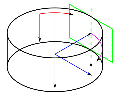
The cylinder is defined in the coordinate system γ (blue) of the image 04 (green) such that:
- cylinder axis is equal to c2 axis of γ,
- image plane of the image 04 is tangential to the cylinder,
- image coordinate system defined on the cylinder surface has square pixels and equal horizontal resolution in the line where it touches the image 04.
This leads that the cylinder has radius = 1 in the γ system. The cylinder surface is a set of points <latex>[x_{\gamma} y_{\gamma} z_{\gamma}]^\top</latex> such that
<latex>x_{\gamma}^2 + z_{\gamma}^2 = 1</latex>
For parametrisation of the cylinder surface we define two coordinate systems: the first (magenta) is based on γ, second (red) is pixel-based system of panoramic image.
First, the surface of the cylinder is parametrised by circumference length (equal to angle since radius=1) and by the <latex>y_{\gamma}</latex> coordinate. The ray <latex>\lambda [x_{\gamma} y_{\gamma} z_{\gamma}]^\top</latex> intersects the cylinder in the point
<latex>\lambda=\frac{1}{\sqrt{x_{\gamma}^2 + z_{\gamma}^2}}</latex>
<latex>[ a_{c\gamma}; y_{c\gamma} ] = [ \mbox{the angle given by } x_{\gamma} \mbox{ and } z_{\gamma}; \frac{y_{\gamma}}{\sqrt{x_{\gamma}^2 + z_{\gamma}^2}} ]</latex>
Second, the pixel size must be applied and image origin adjusted. Since the horizontal pixel size is 1/K(1,1) measured in units given by γ system, this leads to
<latex>[ x_c; y_c ] = K_{11} [ a_{c\gamma}; y_{c\gamma} ] + [x_{0c}; y_{0c} ]</latex>
where the origin <latex>[x_{0c}; y_{0c}]</latex> must be found such that all pixels from the input images will fit into the resulting panorama.
Upload
Upload an archive consisting of:
06_data.mat06_histograms.pdf06_borders.pdf06_panorama.png06_borders_c.pdf06_panorama_c.png- your own images and panorama, if created
- hw06.m – your Matlab implementation entry point.
any other files required by hw07.m (including data and files from the repository).