Table of Contents
Searching in large image databases -- Image retrieval
In the previous labs we were searching for correspondences between image pairs. A disadvantage of this method is its quadratic time complexity in the number of images. In this lab we'll look at image (or object) retrieval – a common problem in many computer vision applications. The goal is to find images corresponding to our query image in a large image database. A naive method – trying to match all pairs – is too slow for large databases. Moreover the set of similar images can be only a tiny fraction of the whole database. Therefore, faster and more efficient methods have been developed. r
1. Image Representation with a Set of Visual Words. TF-IDF Weighting
One of the fastest methods for image retrieval is based on the so called bag-of-words model. The basic idea is to represent each image in a database by a set of visual words from a visual vocabulary. The visual word can be imagined as a representative of an often occurring image patch. With a visual vocabulary, images can be represented by visual words similarly to documents in a natural language.
In the previous labs, the images were represented by a set of descriptions of normalized patches. Visual words can be chosen from a space of such descriptions. Each description can be understood as a point in this space. We'll choose the visual words by vector quantization - one visual word for each cluster of descriptors. We will implement one method commonly used for vector quantization (clustering): K-means.
Vector Quantization - K-means
One of the simplest method for vector quantization is k-means. You should already know this algorithm from the Pattern Recognition course:
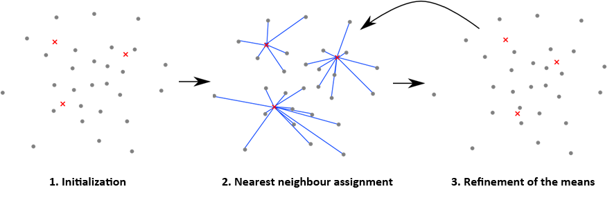
- Initialization: Choose a defined number $k$ of clusters centers (the red crosses in the image). Random points can be chosen from the set of descriptors, but more sophisticated method exists.
- Assign all points to the nearest center – points are assigned to <latex>k</latex> clusters.
- Shift each center into the center of gravity (mean) of the assigned points (compute the center of gravity from points in the same cluster). In the case when the mean has no assigned points a new position has to be chosen for this mean.
Repeat steps 2 and 3 until the assignments in step 2 do not change, or until the global change of point-to-mean distances decreases below some threshold.
Implement k-means.
- Write a function [idxs, dists]=
nearest(means, data), which finds the nearest vector from the set of means (matrix of DOUBLEs with size DxK, where D is the dimension of the descriptor space and K is the number of means) for each column vector in matrix data (of DOUBLEs with size DxN, where N is the number of points). The output of this function are indices idxs (matrix 1xN) of the nearest means and distances dists (matrix 1xN) to the nearest mean. - Write a function [means, err]=
kmeans(K, data), which finds K means in the vector space data and return the sum err of distances between data points and means to which they are assigned.
We prepared the data for you (in the test archive at the bottom of this assignment) to make this assignment a little bit easier.
If we would like to use the functions kmeans and nearest to represent image by visual words, we would do so as follows:
- use
detect_and_describefunction to compute the image descriptors using the same setting for all images and choosing parameters such that there is ca. 2000-3000 descriptors per image in average. - then we apply
kmeansfunction to all descriptors to find e.g. 5000 centers of clusters (means). The cluster centers – vectors in descriptor scape – and their indexes are used as visual words for image representation. The set of clusters (descriptor vectors) is called visual vocabulary. - for image indexing, we assign a visual word index to each image descriptor using
nearestfunction and we store the vector of visual words representing the image to the matrix of cells vw{i}. Similarly, we store matrix of cells geom{i} 6xNi with parameters of frame [x;y;a11;a12;a21;a22] (the rest of the structure pts is not needed), Ni is number of points in i-th image.
Inverted file
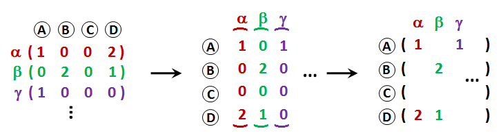
After the previous step, every image is represented by a vector of visual words. By summing the occurrences of the same words we get a vector representation of the image with counts of visual words (see rows <latex>\alpha</latex>,<latex>\beta</latex>,<latex>\gamma</latex> with occurences of words A,B,C,D on the picture below, left). To be able to search effectively in the image database, we need to estimate the similarity. The standard way is to sum the distances of corresponding descriptions. In the bag of words method the vector quantization is used to approximate the description distance. The distance between descriptions is 0 if they are assigned to the same visual word and infinity otherwise. For images represented as vectors of visual words we define similarity as:
<latex>\displaystyle\mathrm{score}(\mathbf{x},\mathbf{y}) = \cos{\varphi} = \frac{\mathbf{x}\cdot \mathbf{y}}{\|\mathbf{x}\|\|\mathbf{y}\|} = \frac{1}{\|\mathbf{x}\|\|\mathbf{y}\|}\sum_{i=1}^D x_i y_i</latex>
where x and y are vectors of visual words (bags of words). We can take advantage of the fact that a part of the similarity can be computed ahead and normalize the size of vectors. After that, the similarity can be computed as a simple dot product of two vectors.
The visual vocabulary can be very big, often with a few thousands or even millions of words. To simplify the distance estimation between such long vectors, the so called inverted file is used. Inverted file is a structure, which for each visual word (A, B, C, D in the picture) contains a list of images <latex>\alpha</latex>,<latex>\beta</latex>,<latex>\gamma</latex> in which the word appears together with the multiplicity.
In Matlab is easy to implement this structure as a sparse matrix. Matlab represents a sparse matrix as column lists of elements. Therefore, our inverted file will be a 2D sparse matrix, where columns are visual words and rows are images. For instance, the third column of the matrix will contain weights of the third word in all images. We compute the weight of the word from its frequency divided by the length of the vector of visual words (i.e. square root of the sum of squared frequencies)
- implement a function
DB=createdb(vw, num_words), which builds the inverted file DB in the form described above (sparse matrix NxM, where N is the number of images and M=num_wordsis number of visual words in the vocabulary. Parameter vw is matrix of cells 1xN, where ith cell contains the list of words in the ith image. (For the sparse matrix, use the Matlab functionsparse.)
TF-IDF weighting
In real images, visual words tend to appear with different frequencies. Similar to words in the text, some words are more frequent than others. The number of visual words in one image is changing depending on the scene complexity and the detector. To deal with these differences, we have to introduce a suitable weighting of visual words. One weighting scheme, widely used also in text analysis and document retrieval, is called TF-IDF (term frequency–inverse document frequency). Weight of each word $i$ in the image $j$ consists from two values:
$$ \mathrm{tf_{i,j}} = \frac{n_{i,j}}{\sum_k n_{k,j}},$$
where $n_{i,j}$ is the number of occurences of word $i$ in image $j$; and
$$ \mathrm{idf_{i}} = \log \frac{|D|}{|\{d: t_{i} \in d\}|},$$
where $|D|$ is the number of documents and $|\{d: t_{i} \in d\}|$ is the number of documents containing visual word $i$. For words that are not present in any image, <latex>\mathrm{idf_{i}}=0</latex>. The resulting weight is:
$$ \mathrm{(tf\mbox{-}idf)_{i,j}} = \mathrm{tf_{i,j}} \cdotp \mathrm{idf_{i}}$$
We need two functions
- a function
idf=getidf(vw, num_words), which computes the IDF of all words based on the lists of words in all documents. The result will be a 1$\times$num_wordsmatrix. - adjust a function
createdbto functionDB=createdb_tfidf(vw, num_words, idf), which instead of word frequencies computes their weights according to TF-IDF (frequencies of each word multiplied by the IDF of the word). Normalize the resulting vectors to 1, as explained above.
Image ranking according to similarity with query image
Thanks to the inverted file we can rank images according to their similarity to the query. The query is defined by a bounding box in the image around the object of interest. With the use of function imrect for rectangle and positions of visual words (first two rows x,y of the cell array geom) take the visual words which are contained inside the rectangle. Compute the length and weights of visual words of the query and multiply it with the corresponding columns of the inverted file, matrix DB. The result is a similarity matrix between the query and database images.
- write a function
[img_ids, score]=query(DB, q, idf), which computes similarity of the query q - list of visual words (1xK matrix, where elements are indexes of visual words) and images in the inverted file DB. Parameter idf are IDF weights of all visual words. The result of this function is an array score with similarities ordered in descending order and img_ids, indexes of images in descending order according to similarities.
What you should upload?
Functions nearest.m, kmeans.m, createdb.m, createdb_tfidf.m a query.m together with all used non-standard functions you have created.
Testing
To test your code, you can use a matlab script and a function 'publish'. Copy tfidf_test.zip and unpack it to direcotry which is in matlab paths (or put it into directory with your code) and execute. Compare your results with ours.
2. Fast spatial verification. Query expansion.
After image ranking according to vector similarities, we find the set of images, which have common words with the query. In an ideal case, we will find several views of the same scene. We know that the visual words are representing parts of the scene in the image. Therefore, the coordinates of the visual words in images of the same scene are spatially related. This relation is defined by the mutual position of the scene and the camera at the moment when the images were taken. We can use this relation to verify, if the images really contain the same scene or object.
Spatial verification
The tentative correspondences of visual words will be needed for spatial verification. They will be used to discover a geometric transformation between the coordinates of visual words from the query and words from each relevant image.
After ordering according to tf-idf, we have a set of relevant images. These are images, which have at least several visual words common with the query. For each pair, query and a similar image, we find tentative correspondences. Same visual words represent features with similar descriptions, but there can be several features with the same visual words in one image and we have to try each pair because we do not have the original description anymore. If there is M features with the same particular visual word in the query image and N features with the same word in a similar image, the tentative corresponding pairs (pairs of word indexes in the image) will be a Cartesian product of the feature sets. We treat each visual word in the image this way. There may be a lot of features with the same visual word in both images, which produces a large number of tentative pairs (NxM), from which only min(N,M) can be true correspondences. For this reason we will set two constraints on the total number of tentative correspondence in each image pair (max_tc) and the maximal number of pairs (max_MxN). Moreover, to control the number of tentative correspondences we will prefer the visual words with smaller product NxM.
- write a function
corrs=corrm2m(qvw, vw, relevant, opt), which computes tentative correspondences and stores them to an array of cells corrs (1xKof type CELL). Each cell will hold an array 2xTk of pairs of visual word indexes in the images (first image is query, second is a similar image from the database). Input is a vector of visual words qvw (matrix 1xQ of type DOUBLE) in query image; array of cells vw with list of visual words in images in the database; matrix relavant (1xK of type DOUBLE) the list of indexes of relevant images. Finally opt is a structure with two fields max_tc and max_MxN.
We need a geometric model for the verification tentative correspondences. In the same manner as in the previous task, we can use a homography or an epipolar geometry, but the verification of a huge amount of images can be too time consuming. It happens quite often that only a small fraction of tentative correspondences are true correspondences. Therefor it is more feasible to take a simpler model. We can use the fact that our feature points are not only points but affine (resp. similarity) frames. Remember that a frame defines a geometric relation between canonical frame and an image. If we compose an affine (resp. similarity) transformation from query image into canonical frame and from canonical frame into relevant image from the database, we will get an affine (resp. similarity) transformation of visual word neighborhood from the query image to the image from the database.
It is clear that geometric transformation between the query and the image from database is not necessarily affine (resp. similarity), but from the assumption that we deal with a planar object, we can take it as local approximation of perspective transformation. With a big enough threshold we can consider all “roughly” correct points to be consistent. The advantage of this method is its speed. From each tentative correspondence we get a hypothesis of transformation – it is not necessary to use sampling. This way, we can verify all hypotheses for each pair query–database image and save the best one. The number of inliers will be the new score, which we will use for the reordering of relevant images.
- write a function
[scores, A]=ransacm2m(qgeom, geom, corrs, relevant, opt), which estimates the number of inliers and the best hypothesis A of transformation from query to database image. Input is an array qgemo (6xQ of type DOUBLE, where Q is the number of words in the query) of geometries (affine frames [x;y;a11;a12;a21;a22]) of query visual words; array of cells geom with geometries (see image_indexing above) of images from the database; array of cells corrs and a list of relevant images relevant as in the previous function. The function returns an array scores (of size 1xK and type DOUBLE) with the numbers of inliers and a matrix of transformations A (matrix 3x3xK) between query and database image. Structure opt contains a field threshold - maximal euclidean distance of the reprojected points.
- join the spatial verification with tf-idf voting into one function
[scores, img_ids, A]=querysp(qvw, qgeom, bbx, vw, geom, DB, idf, opt), which orders images from database according to number of inliers. The result will be output of functionransacm2mjoined with output of functionquery. Score of relevant images will be added to score from functionquery. Transformations A for other images will be set to a zero matrix 3×3. img_ids will be the ordered list of image indexes according to the new score. Input parameters will be the same as described above, with one expception – parameters qvw and qgeom will contain all visual words from the query and parameter bbx (a bounding box in form [xmin;ymin;xmax;ymax]) which will be used for visual word selection. Parameter opt will contain the union of parameters for functionsransacm2mandcorrm2m, maximal number of images for spatial verification (maximal length of parameter relevant) will be set in field max_spatial.
Query expansion
(optional task for 2 bonus points)
The basic idea of query expansion is to use a knowledge of spatial transformation between query and database image, for enriching the set of visual words of the query. In the first step, correct images (results) for the first query have to be chosen. To avoid expansion of unwanted images, it is necessary to choose only images which are really related to query image. This can be done by choosing only images with high enough score (for instance at least 10 inliers). For each chosen image the centers of visual words are projected by transformation A-1 and words which are projected inside the query bounding box are added into the query. It is good idea to constrain the total number of visual words in the expanded query. It is desirable to choose visual words, which add information (it is useless to add a visual word from each image with frequency 100, it will only cause problem during correspondence finding). Therefor the words are ordered according to tf and then the first max_qe words are chosen.
- add query expansion to the function
[scores, img_ids, A]=querysp(qvw, qgeom, bbx, vw, geom, DB, idf, opt). Query expansion will be used if the parameter opt.max_qe will exist and will be non-zero. The other parameters are the same.
Testing
To test your code, you can use a matlab script and a function 'publish'. Copy spatial_test.zip and unpack it to direcotry which is in matlab paths (or put it into directory with your code). Copy the file with mpvdb_haff2.mat database, unpack archive with images and execute the test script. Compare your results with ours.
Your task: image retrieval in big databases
On the set of 1499 images (225 images by your colleagues from a previous year, 73 images of Pokemons, 506 images from dataset ukbench) and 695 images from the dataset Oxford Buildings) we have computed features with detector sshessian with Baumberg iteration (haff2, returns affine covariant points). We have estimated dominant orientation and computed SIFT descriptors. With k-means algorithm (with approximate NN) we have estimated 50000 cluster centers from SIFT descriptions and we have assigned all descriptions. You can find the data in file mpvdb50k_haff2.mat, where array of cells with the lists of visual words is stored in variable VW, array of cells with geometries in variable GEOM and names of the images in the variable NAMES. Cluster centers are stored in file mpvcx50k_haff2.mat in variable CX. Compressed images are in file mpvimgs1499.zip. Descriptions to images are in file mpvdesc_haff2.mat, stored as array of cells DESC. Elements of these cells are matrices of type UINT8 of size 128xNi, where Ni is number of points in ith image. Compute results on the database of haff2 detector (it should work better for more difficult perspective transformation).
Choose 20 images:
- 10 from Oxford Buildings dataset
- 5 Pokemons: X=(your index in class MPV)-1, your images are those with index from (2*X+1) to (2*X+5).
- 5 from dataset ukbench.
Save their indexes into variable query_id. Assign decription with function nearest. On each image chose rectangle with object of query (for instance with function imrect) and save coordination (not indexes! The top-left corner has coordination (0,0)) into column of matrix query_bbx of size 4×20 of type DOUBLE in order [xmin;ymin;xmax;ymax]. Choose visual words, which have centers inside the bounding box (including boundary). With function querysp query the database and store the results (score, list of images and transformation A) into structure query_results in correct position (1..20) into fields score, img_ids, A. All variables query_* and variable opt save into file results.mat and submit into upload system as task 07_results.
Archive the functions kmeans.m, nearest.m, createdb.m, createdb_tfidf.m, query.m, corrm2m.m, ransacm2m.m and querysp.m together with all used non-standard functions you have created (add the functions from first lab only if they are needed in this task) into one file and submit to as task 07_spatial.